Cruise Control Example

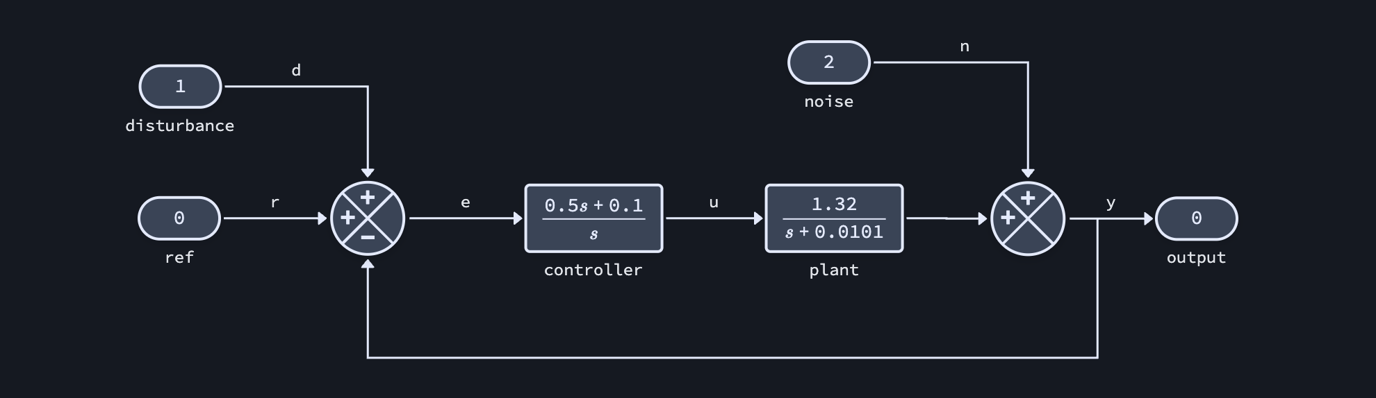
This example demonstrates a simple feedback control system with a proportional-integral controller and first-order plant. It is borrowed from the “cruise control” example in Åström & Murray, Chapter 3.

System Overview

The plant models a transfer function from engine throttle to speed and is derived from linearizing a 1D nonlinear model about a particular engine gear and vehicle speed.

The linearized plant model is:

\[ G(s) = \frac{b}{s - a}, \qquad b=1.32, ~~ a=-0.0101 \]

and this can be controlled with simple proportional-integral (PI) feedback:

\[ C(s) = k_p + \frac{k_i}{s}, \qquad k_p = 0.5, ~~ k_i = 0.1 \]

Setup

Show code cell content

Hide code cell content

# ruff: noqa: N802, N803, N806, N815, N816

import matplotlib.pyplot as plt
import numpy as np

import control

import lynx

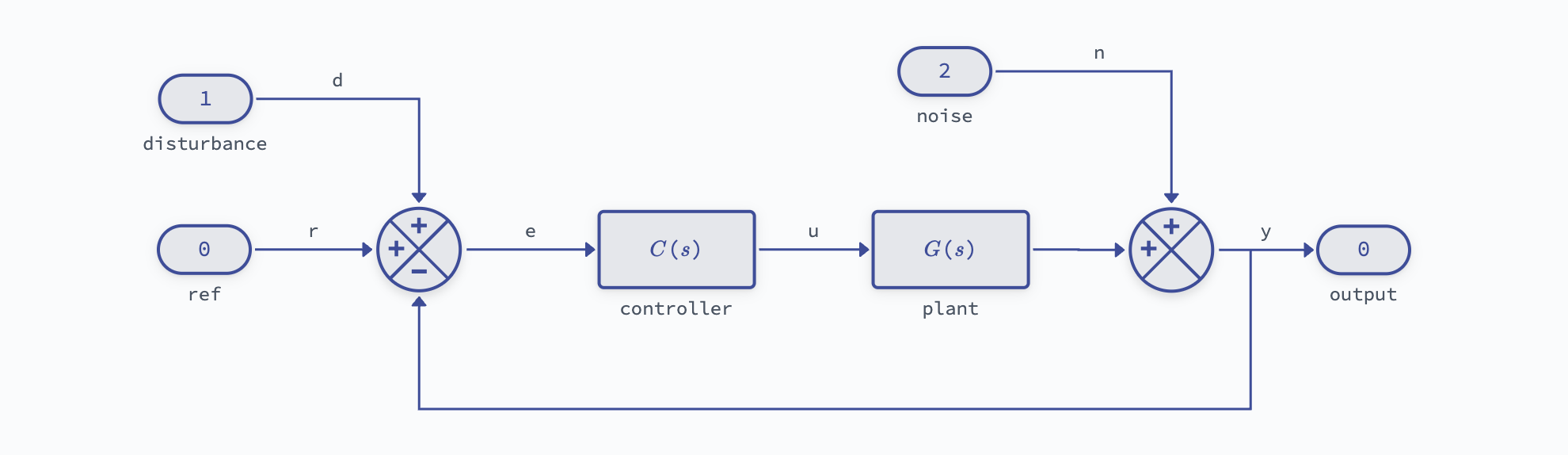
Create Diagram

It is possible to create this diagram programmatically using the block diagram API; however, you can expect a generally poor experience programmatically constructing block diagrams.

Instead, either use the interactive widget to construct the diagram yourself, or load one of the pre-built templates and modify the block parameters.

For a simple feedback controller with a transfer function plant model we can load the "feedback_tf" template:

# Construct a new diagram from scratch:
# diagram = lynx.Diagram()
# lynx.edit(diagram)

# Load the diagram architecture from a template
diagram = lynx.Diagram.from_template("feedback_tf")

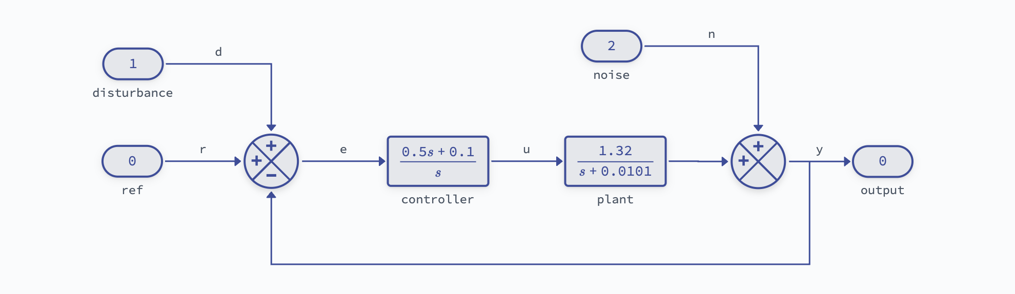
Update the transfer functions and turn off custom LaTeX rendering to see the numerical values:

# Linearized vehicle model
b = 1.32
a = -0.0101
diagram["plant"].set_parameter("num", [b])
diagram["plant"].set_parameter("den", [1, -a])
diagram["plant"].custom_latex = None

# PI controller
kp = 0.5
ki = 0.1
diagram["controller"].set_parameter("num", [kp, ki])
diagram["controller"].set_parameter("den", [1, 0])
diagram["controller"].custom_latex = None

Export to Python-Control

Extract the closed-loop transfer functions from r to u and y as a python-control TransferFunction object:

# Export closed-loop transfer functions
G_yr = diagram.get_tf('r', 'y')
G_ur = diagram.get_tf('r', 'u')

print(f"Closed-loop transfer function:")
print(G_yr)

Closed-loop transfer function:
<TransferFunction>: sys[4]$indexed$converted
Inputs (1): ['ref']
Outputs (1): ['sum_1769105068595']

      0.66 s + 0.132
  ----------------------
  s^2 + 0.6701 s + 0.132

Then these subsystems can be further analyzed using any of the python-control tools.

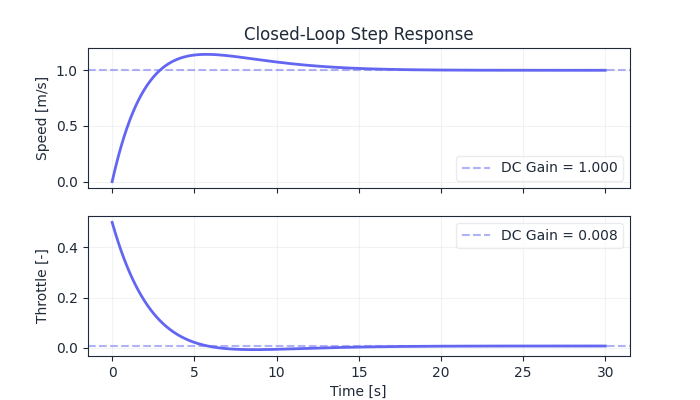
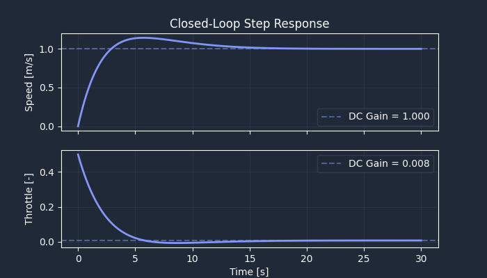
For instance, to evaluate the step response:

# DC gains
yr_dcgain = control.dcgain(G_yr)
ur_dcgain = control.dcgain(G_ur)

# Compute step responses
t = np.linspace(0, 30, 500)
_, y = control.step_response(G_yr, t)
_, u = control.step_response(G_ur, t)

Show code cell content

Hide code cell content

fig, ax = plt.subplots(2, 1, figsize=(7, 4), sharex=True)

ax[0].plot(t, y, linewidth=2)
ax[0].axhline(y=yr_dcgain, linestyle='--', alpha=0.5, label=f'DC Gain = {yr_dcgain:.3f}')
ax[0].grid(True, alpha=0.3)
ax[0].set_ylabel('Speed [m/s]')
ax[0].set_title('Closed-Loop Step Response')
ax[0].legend()

ax[1].plot(t, u, linewidth=2)
ax[1].axhline(y=ur_dcgain, linestyle='--', alpha=0.5, label=f'DC Gain = {ur_dcgain:.3f}')
ax[1].grid(True, alpha=0.3)
ax[1].set_ylabel('Throttle [-]')
ax[1].legend()

ax[-1].set_xlabel('Time [s]')
plt.show()