Physical system
In this first part of the series, we will begin our development process by specifying the physical system, including the motor, driver circuit, and microcontroller board. The problem we will be trying to solve is position control - determining a voltage signal to quickly and smoothly achieve a desired orientation of the output shaft. This type of control may be easily adapted to force or speed control, and can be a building block in more complex multi-joint robotics applications.
The entire system may be built for less than $200 USD, including a pair of STM32 development boards that are suitable for a wide range of other applications. Alternatively, you can skip the DIY build and simply follow along with the code; all referenced data will be linked to as needed.
Note that none of the links below are “affiliate” links and we have no financial interest in what parts you buy - any recommendations below are just based on our experiences with the components.
DC gearmotor
An electric motor converts electrical to mechanical energy. This particular model is a 47:1 brushed DC gearmotor from Pololu, meaning that the particular arrangement of permanent magnets, electromagnets and brushes allows it to run continuously using a steady DC voltage. This model also has a built-in quadrature encoder, enabling us to precisely determine the shaft position by counting the encoder pulses.
An idealized physics model of such a motor represents the electrical component as an RL circuit, and the mechanical component as damped rotational motion coupled via a linear torque/back EMF relationship:
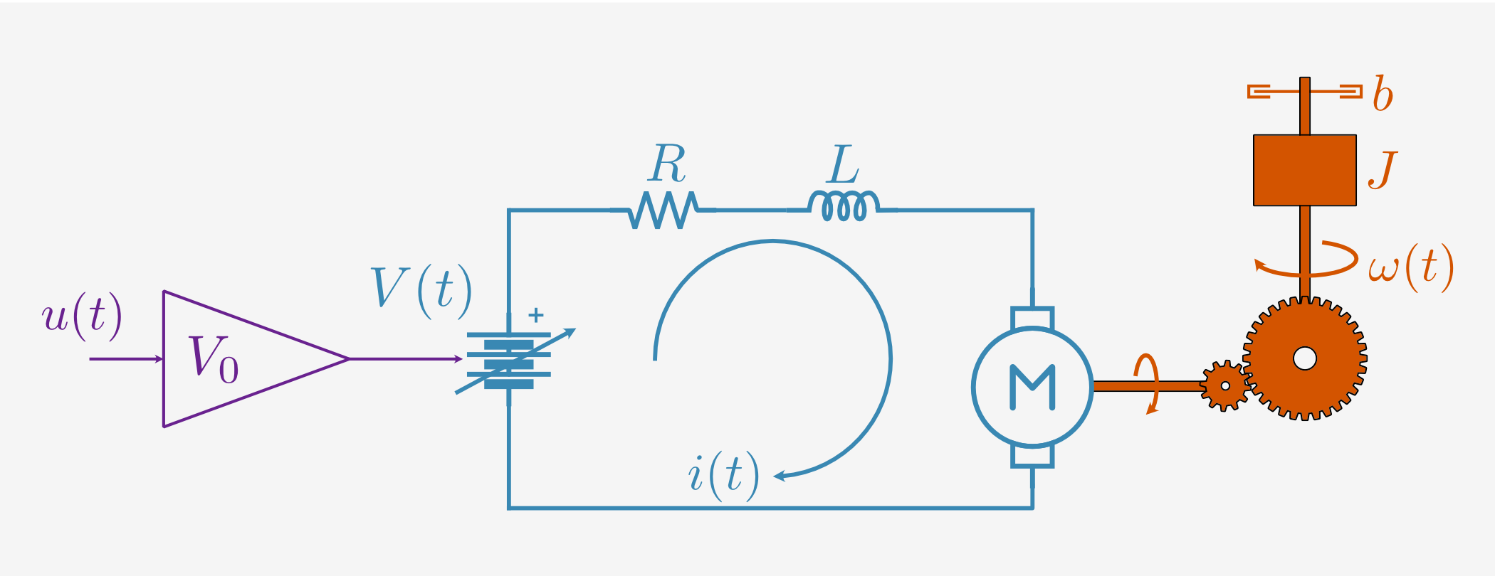
The current \(i(t)\) through the RL loop responds to applied voltage \(V(t)\), activating the electromagnets and producing both a torque on the motor shaft and a back EMF in the electrical circuit. The motor shaft is connected to the output shaft via a planetary gear with ratio \(G\), resulting in a scaled torque on the output shaft, which is moving with angular velocity \(\omega(t)\).
For inductance \(L\), resistance \(R\), back EMF constant \(k_\mathcal{E}\), gear ratio \(G\), effective rotational inertia \(J\), and viscous damping constant \(b\), the ideal governing equations are:
Of course, the output shaft position \(\theta(t)\) is simply the integrated angular velocity: \(\dot{\theta} = \omega\). This model neglects more complex phenomena like backlash and Coulomb friction, but as we will see, it is sufficiently accurate for our purposes. Without these effects, the model is purely linear and can be written as a transfer function from applied voltage \(V(s)\) to position \(\theta(s)\):
The poles of this transfer function indicate two time constants: an electrical constant \(\tau_e = L / R\) (around 1 ms) and a mechanical one \(\tau_m = J / b\) (around 100 ms).
Motor driver circuit
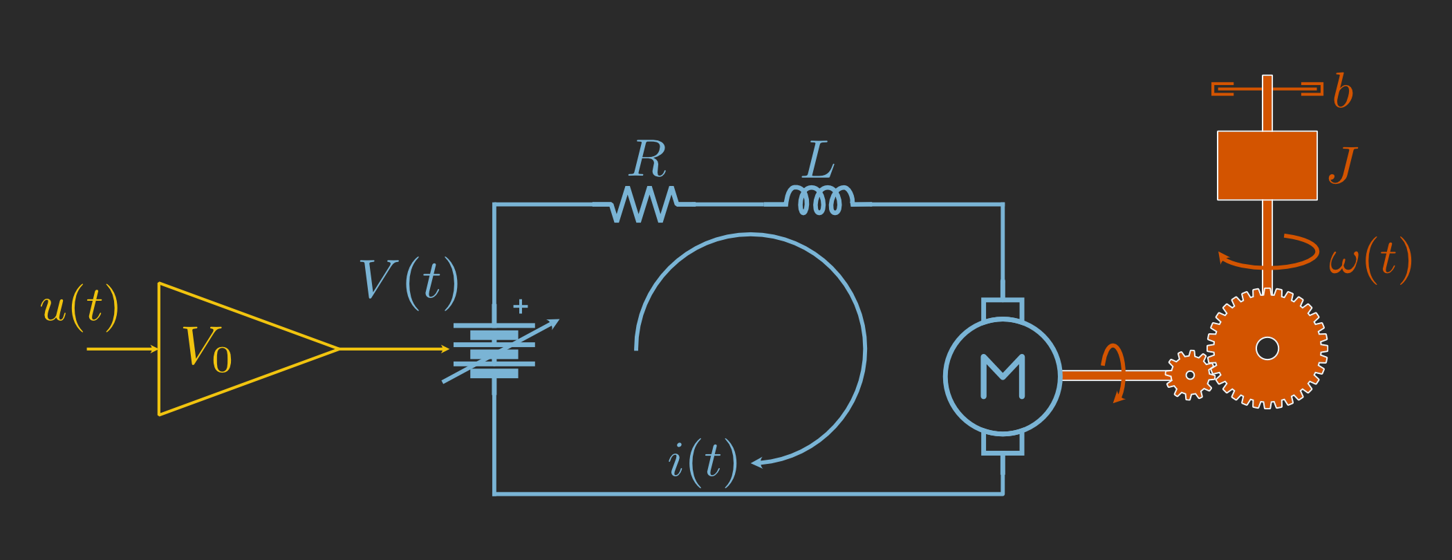
Brushed DC motors are relatively simple to operate, but they do require some “driver” electronics, typically at least an H-bridge circuit to switch a higher-voltage power supply using the logic-level PWM signal and to invert polarity for speed reversals.
As shown by the diagram above, we will model the H-bridge driver mathematically as a simple linear gain from the pulse width modulation (PWM) duty cycle \(u(t)\) to applied voltage \(V(t)\) based on nominal supply voltage \(V_0\). Again, for our purposes this is a reasonably accurate model, though it does neglect high-frequency switching, MOSFET effects, etc.
The driver used in this tutorial is also a Pololu model: the VNH5019 motor driver carrier board. While more expensive than a bare H-bridge, this board has some protection features that make it robust to off-nominal voltage, current, and temperature levels (not always uncommon during prototyping!). It also has built-in current sensing, with a pin that outputs an analog voltage proportional to motor current. This is useful for characterization (see Part 2), debugging, direct torque control, and the current control loop of a cascaded position or speed controller.
In addition to the built-in current output, we will also directly measure the voltage on the output side of the driver via voltage dividers and simple RC filters (to smooth out the PWM switching). The full circuit is shown below.
The last piece of the circuit is the power supply. Here we will use a simple 12V “wall wart” supply - more on that in Part 5.
Microcontroller
The circuit described above will effectively translate a PWM signal into a modulated supply voltage to power the motor, as well as arranging for measurements of current, voltage, and shaft position. Responsibility for producing the PWM signal, the logic outputs to enable the H-bridge and control direction, performing A/D conversion on the sensor voltages, and actually running the control algorithm all falls to the microcontroller (MCU).
For this tutorial we will use the Nucleo-F439ZI STM32 dev board, a versatile and relatively powerful board running an ARM Cortex M4 processor and with a number of convenient features for this application:
180 MHz clock speed (more than enough for a 10 kHz control loop)
PWM generation + motor control features like dead time insertion
Built-in functionality for counting quadrature encoder pulses
Plenty of A/D bandwidth, including hardware triggering and DMA for deterministic timing
Built-in debugger/programmer + USB link (we’ll use for sending data back to the computer)
[Optional]: Building the system
The following are some notes to help with building the project; if you just want to follow along with the Python code, feel free to skip this part.
Component list
Nucleo-F439ZI STM32 dev board - buy at least two if you want to do HIL testing
Breadboard and hookup wire
Assorted resistors and capacitors
A button or switch to trigger control/test sequences
Circuit diagram
Here’s the full motor control circuit, including current, voltage, and position sensing:
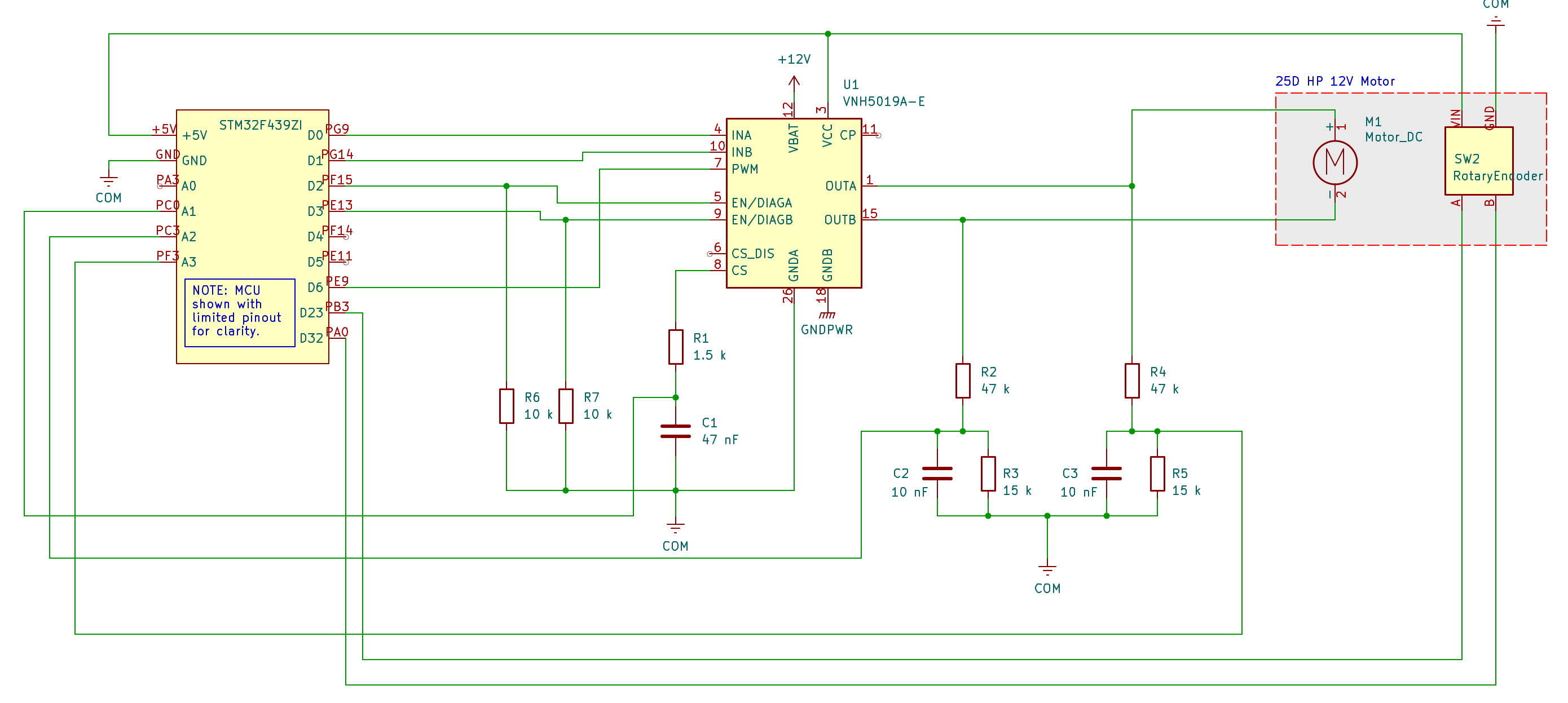
A KiCad schematic is also available on GitHub.
The only feedback signal that’s used in the final controller is position, so if you want to skip the characterization step you can simplify the circuit considerably by removing all the sensor circuitry except for the quadrature encoder.
For HIL testing, the circuit is similar, but all the physical hardware is replaced by a second Nucleo board running a real-time simulation:
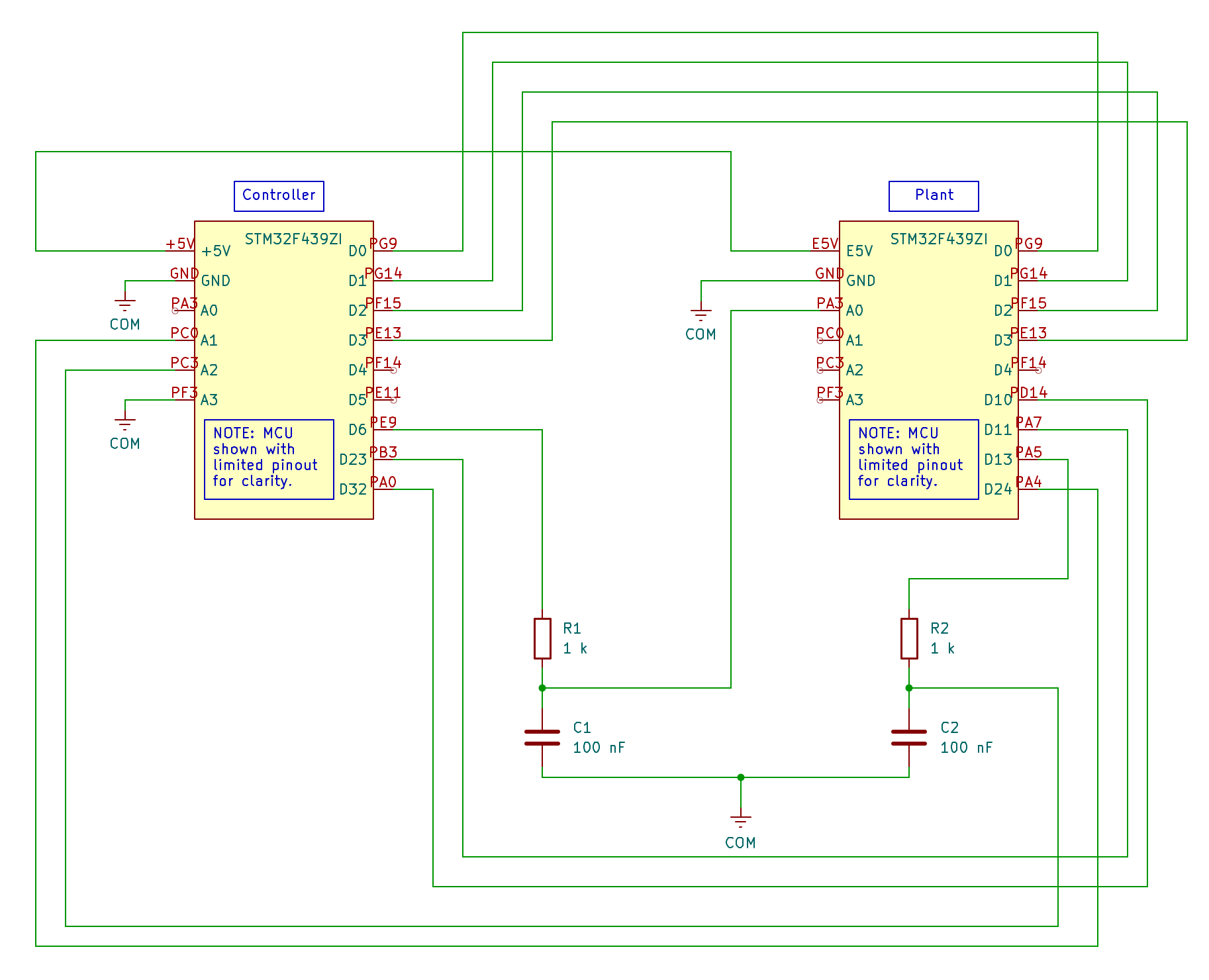
The HIL test is another optional step, but as we will see, it is very convenient for troubleshooting and rapidly iterating the control algorithm.
Deployment toolchain
We’ve used the following set of tools (all free):
STM32CubeMX to configure the MCU and peripherals
CMake to build
ARM GCC toolchain for cross-compilation
OpenOCD for flashing the firmware
You can of course adapt this to whatever tools you are familiar with. Cortex-Debug is also a useful VSCode extension for debugging (set breakpoints, inspect variables, etc.), though we won’t discuss this in this series.
To install these tools:
Mac
brew install cmake
brew install --cask gcc-arm-embedded
brew install openocd
Linux (Debian/Ubuntu)
sudo apt install cmake
sudo apt install gcc-arm-none-eabi
sudo apt-get install openocd
Test with:
arm-none-eabi-gcc --version
cmake --version
# With board plugged into USB:
openocd -f interface/stlink.cfg -f target/stm32f4x.cfg
Each application destined for deployment to an STM32 will have its own “project” stored in subfolders in the _static/ directory. We will autogenerate the controller and plant model code using Archimedes, but the “main” application will still be a combination of autogenerated peripheral configuration code (from CubeMX) and runtime code to call our Archimedes-generated functions.
To build and deploy a project:
cd project_name
cmake --preset=Release
cmake --build --preset=Release
openocd -f interface/stlink.cfg -f target/stm32f4x.cfg \
        -c "program build/Release/<project_name>.elf verify reset exit"