Flight Dynamics¶

After Part 1, we now have a validated implementation of the Stevens-Lewis-Johnson F-16 model that’s compatible with Archimedes for ODE solving, autodiff, trajectory optimization etc.

In this part we’ll take a hierarchical approach, defining the flight dynamics model with nested subsystems - something like a Python version of Reference and Variant Subsystems in Simulink. For much more on the “why” and “how” of this, see the tutorials on Structured Data Types and Hierarchical Modeling. This structure can be reused for many conventional fixed-wing aircraft, and with light modifications can be adapted to a wide variety of other vehicle dynamics models as well.

Subsystem Models¶

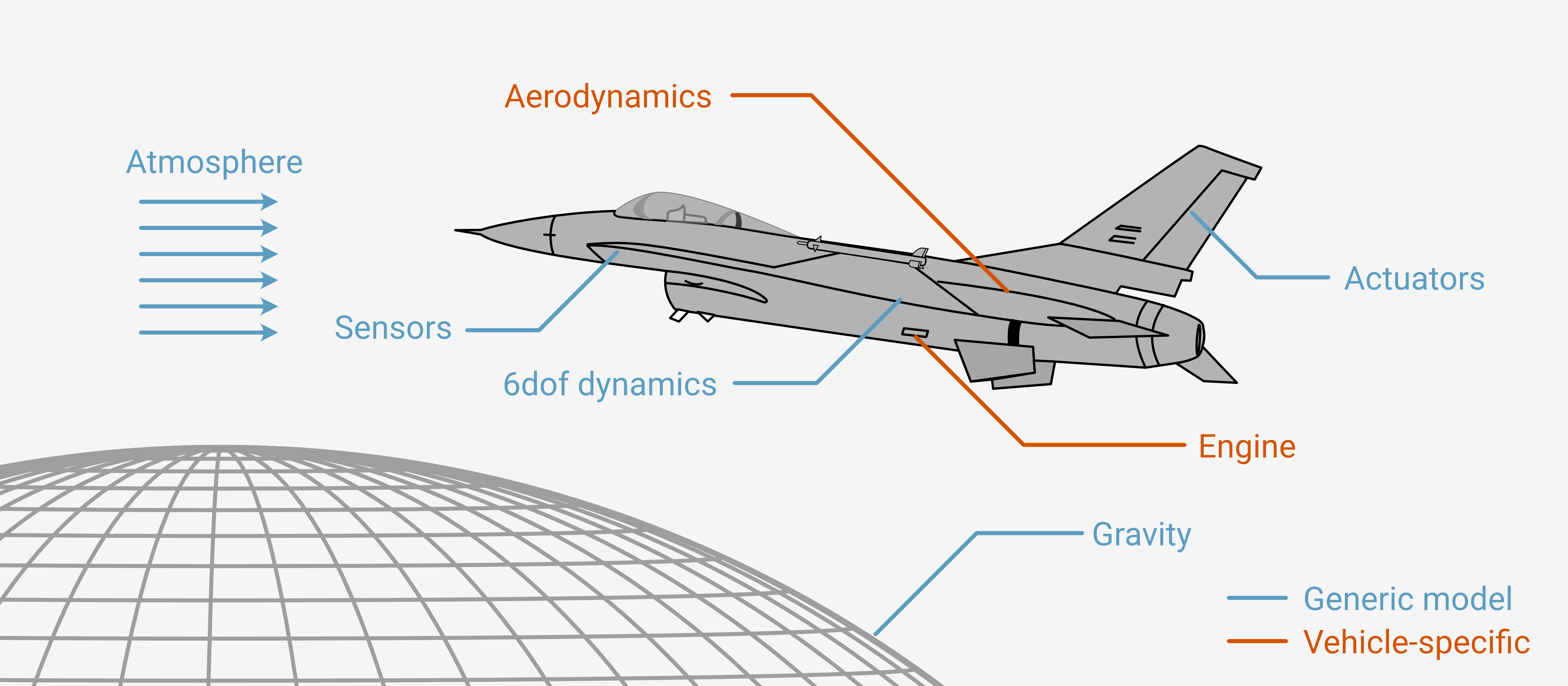
So, what’s in an F-16? We’ll consider a number of “subsystems”:

SubsonicF16
├── RigidBody
├── GravityModel
├── AtmosphereModel
├── F16Engine
├── F16Aero
└── Actuator (x3)

Sensors are obviously important to model as well, but we’ll just be looking at basic vehicle stability and response, so we won’t include these for now.

Following the hierarchical dynamics modeling design pattern, we will first create an abstract base class or Protocol for each of these subsystems that clearly defines their inputs and outputs. Then we can add dynamic state to each concrete implementation as necessary.

We’ll build up the interface definitions first, then see a couple of concrete implementations, and finally see how it fits together for the full vehicle model. We won’t go through all the subsystems in detail - just enough to get the general idea. As always, the full source code is on GitHub.

At a high level, each of these subsystem models will adhere to one of two common interfaces (following the ideas in the Hierarchical Design Patterns tutorial series).

For simple “callable” components that will never be stateful (gravity and atmosphere), the subsystem will look like the following:

@struct
class CallableSubsystem:
    parameter: float

    def __call__(self, *args, **kwargs):
        """Evaluate the component model (stateless algebraic function)"""

Subsystems that act like state-space models will have a more complex interface that clearly defines structured input, output, and dynamic state types:

@struct
class DynamicSubsystem:
    parameter: float
    
    @struct
    class Input:
        ...  # Define fields of the subsystem inputs

    @struct
    class Output:
        ...  # Define fields of the subsystem outputs

    @struct
    class State:
        ...  # Define dynamic state fields, or "pass" for empty state

    def dynamics(self, t: float, x: State, u: Input) -> State:
        ... # Calculate time derivatives, or "return x" if component model has no state

    def output(self, t: float, x: State, u: Input) -> Output:
        ... # Calculate subsystem outputs

This pattern lets us predictably and safely pass data between components and define different model variants of a particular subsystem. Providing placeholders for state and dynamics also makes it easy to switch between idealized models (pure feedthrough) and higher-fidelity models with internal dynamics.

Let’s start simple: gravity.

Gravity¶

Here we just need to compute the gravitational acceleration vector as a function of position. There’s nothing complicated about this, and it doesn’t require a state, so we can use a simple callable Protocol to define the interface:

class GravityModel(Protocol):
    def __call__(self, p_E: np.ndarray) -> np.ndarray:
        """Gravitational acceleration at the body CM in the earth frame E

        Args:
            pos: position vector in the earth frame E [ft]

        Returns:
            g_E: gravitational acceleration in earth frame E [ft/s^2]
        """

This already gives us a lot of flexibility - we could model a spherical potential, oblate Earth, perturbations, etc. It’s not totally general, but for the purposes of F-16 flight we’re pretty well covered.

In fact, our main gravity model implementation will be even simpler:

@struct
class ConstantGravity:
    """Constant gravitational acceleration model

    This model assumes a constant gravitational acceleration vector
    in the +z direction (e.g. for a NED frame with "flat Earth" approximation)
    """

    g0: float = GRAV_FTS2  # ft/s^2

    def __call__(self, p_E):
        return np.hstack([0, 0, self.g0])

Note

A reminder about Protocol types in modern Python - these are a way to define the behavior of classes. They’re not directly inherited from, but because we’ve written ConstantGravity to implement the GravityModel interface, type hints and static type checking will work if we say some argument will be a GravityModel and then pass it ConstantGravity. More importantly for our purposes, this helps create well-defined interfaces between subsystems.

For “meatier” subsystems where we actually want inheritance behavior, abstract base classes are often a better choice to define the interface.

Atmosphere¶

Atmosphere we can handle similarly. For flight dynamics we mainly want an atmosphere model that will compute Mach number and dynamic pressure as a function of “true” (wind-relative) airspeed and altitude. This is easily encapsulated in another Protocol:

class AtmosphereModel(Protocol):
    def __call__(self, Vt: float, alt: float) -> tuple[float, float]:
        """Compute Mach number and dynamic pressure at given altitude and velocity.

        Args:
            Vt: true airspeed [ft/s]
            alt: altitude [ft]

        Returns:
            mach: Mach number [-]
            qbar: dynamic pressure [lbf/ft²]
        """

The atmosphere model used in the reference implementation assumes an ideal gas in hydrostatic equilibrium with a linear temperature gradient. We’ll call it LinearAtmosphere for short:

@struct
class LinearAtmosphere:
    """
    Linear temperature gradient atmosphere model using barometric formula.

    Density varies as ρ = ρ₀(T/T₀)^n where n = g/(R·L) - 1
    for a linear temperature profile T = T₀(1 - βz).
    """

    g0: float = 32.17  # Gravitational acceleration [ft/s²]
    R0: float = 2.377e-3  # Density scale [slug/ft^3]
    gamma: float = 1.4  # Adiabatic index for air [-]
    Rs: float = 1716.3  # Specific gas constant for air [ft·lbf/slug-R]
    dTdz: float = 0.703e-5  # Temperature gradient scale [1/ft]
    Tmin: float = 390.0  # Minimum temperature [R]
    Tmax: float = 519.0  # Maximum temperature [R]
    max_alt: float = 35000.0  # Maximum altitude [ft]

    def __call__(self, Vt, alt):
        L = self.Tmax * self.dTdz  # Temperature gradient [°R/ft]
        n = self.g0 / (self.Rs * L) - 1  # Density exponent [-]
        Tfac = 1 - self.dTdz * alt  # Temperature factor [-]
        T = np.where(alt >= self.max_alt, self.Tmin, self.Tmax * Tfac)
        rho = self.R0 * Tfac**n
        mach = Vt / np.sqrt(self.gamma * self.Rs * T)
        qbar = 0.5 * rho * Vt**2
        return mach, qbar

For completeness, the source code also implements the US Standard Atmosphere 1976 model. The two are nearly identical in a particular altitude band, but the USSA1976 model is valid over a much wider altitude range.

Actuators¶

The control surface actuator components model the electrical-mechanical-hydraulic system that produces deflections in the control surfaces. We’ll consider these to be single-input, single-output (SISO) systems mapping from commanded position \(u\) to actual position \(y\) (in this case, both measured in degrees).

Here we will depart from the Protocol approach and define a base class, since there is some default behavior that we’d like the classes to inherit. The base class is stateless, and requires at a minimum that children implement the output method:

class Actuator(metaclass=abc.ABCMeta):
    """Abstract base class for SISO actuator components."""

    @struct
    class State:
        pass  # No state by default

    def dynamics(self, t: float, x: State, u: float) -> State:
        """Compute the actuator state derivative."""
        return x

    @abc.abstractmethod
    def output(self, t: float, x: State, u: float) -> float:
        """Compute the actuator output."""
        pass

    def trim(self, command: float) -> State:
        """Return a steady-state actuator state for the given command."""
        return self.State()

The simplest actuator model is direct linear feedthrough: \(y = u\). That is, the ideal model assumes that the commanded position is realized instantaneously. We can implement this with a gain for a little more flexibility, though in this formulation the gain will always be 1:

@struct
class IdealActuator(Actuator):
    """Ideal actuator with instantaneous linear response."""

    gain: float = 1.0

    def output(self, t: float, x: Actuator.State, u: float) -> float:
        return self.gain * u

As with the base class, this model is “stateless”. More precisely, it has an empty state (Actuator.State) that we’ll pass around as a placeholder for compatibility with stateful models.

In reality, of course, the control surfaces can’t respond instantaneously. A common way to model the real response is with a rate- and position-limited first-order lag. This can be a bit tricky to implement as a smooth ODE; technically we should be defining zero-crossing events to handle position and velocity saturation. However, CVODES can handle \(C^0\)-smooth right-hand side functions fairly robustly, so the following model works:

@struct
class LagActuator(Actuator):
    tau: float
    gain: float = 1.0
    rate_limit: float | None = field(static=True, default=None)
    pos_limits: tuple[float, float] | None = field(static=True, default=None)

    @struct
    class State(Actuator.State):
        position: float = 0.0

    def dynamics(self, t: float, x: State, u: float) -> State:
        # Compute desired rate
        cmd, pos = u, x.position
        rate = (self.gain * cmd - pos) / self.tau

        # Apply rate limit
        if self.rate_limit is not None:
            max_rate = self.rate_limit
            rate = np.clip(rate, -max_rate, max_rate)

        if self.pos_limits is not None:
            min_pos, max_pos = self.pos_limits
            rate = np.where((pos <= min_pos) * (rate < 0.0), 0.0, rate)
            rate = np.where((pos >= max_pos) * (rate > 0.0), 0.0, rate)

        return self.State(rate)

    def output(self, t: float, x: State, u: float) -> float:
        pos = x.position
        if self.pos_limits is not None:
            min_pos, max_pos = self.pos_limits
            pos = np.clip(pos, min_pos, max_pos)
        return pos

    def trim(self, command: float) -> State:
        pos = command
        if self.pos_limits is not None:
            min_pos, max_pos = self.pos_limits
            pos = np.clip(pos, min_pos, max_pos)
        return self.State(position=pos)

The rate limits can add significant effective lag into the system for aggressive changes in deflection. For instance, here is the step response of the F-16 elevator using the parameters in Appendix A.4 of Stevens, Lewis, and Johnson:

The output of these actuator models will be fed to the aerodynamics model as the actual control surface deflections.

Incidentally, this is a pretty good illustration of why it’s important to have a healthy phase margin - the rate limiting is a nonlinear effect that would be missed by a stability analysis, leading to a significant underestimate of lag in the actuator subsystem.

Rigid Body Dynamics¶

The next “subsystem” is an odd one. RigidBody is fully generic, meaning that unlike the aircraft-specific aerodynamics and engine models, or even the Earth-specific gravity model, RigidBody doesn’t really know or care anything about the body that it’s simulating. In fact, we don’t even need to actually instantiate it - the pieces we need are all class attributes or methods. RigidBody.dynamics simply takes forces, moments, and inertia characteristics and calculates the time derivatives of the position, attitude, velocity, and angular velocity.

Because it is generic and applicable across engineering domains, this class is built into the spatial module of Archimedes. For more on RigidBody see the blog post introducing the spatial module.

For now, all we really need to know is how the State and dynamics of the RigidBody subsystem are defined:

class RigidBody:
    """6-dof rigid body dynamics model"""

    @struct
    class State:
        pos: np.ndarray  # Position of the center of mass in the world frame
        att: Attitude  # Attitude (orientation) of the vehicle
        vel: np.ndarray  # Velocity of the center of mass in body frame B
        w_B: np.ndarray  # Angular velocity in body frame (ω_B)

    @classmethod
    def dynamics(cls, t: float, x: State, u: Input) -> State:
        """Calculate 6-dof dynamics"""

This will become an integral part of the final vehicle model.

Engine and Aerodynamics¶

The final two subsystems are the most unique to the F-16 - and also the most complex. When building custom flight dynamics models, usually the bulk of the work goes into getting these subsystems right.

The details of these models are therefore not likely to be of broad interest (though the source code is on GitHub). However, we can understand the role that each of them play by defining their interface as a Protocol:

class F16Engine(Protocol):
    """F-16 engine model"""

    @struct
    class Input:
        throttle: float  # Throttle position [0-1]
        alt: float  # Altitude [ft]
        mach: float  # Mach number

    @struct
    class Output:
        thrust: np.ndarray  # Thrust magnitude [lbf]

    @struct
    class State:
        ...

    def dynamics(self, t: float, x: State, u: Input) -> State:
        """Time derivative of engine model state"""

    def output(self, t: float, x: State, u: Input) -> Output:
        """Calculate engine thrust output"""

    def trim(self, throttle: float) -> State:
        """Calculate trim conditions for the engine model"""


class F16Aero(Protocol):
    @struct
    class Input:
        condition: FlightCondition  # Flight condition
        w_B: np.ndarray  # Angular velocity in body frame (ω_B) [rad/s]
        elevator: float  # Elevator deflection [deg]
        aileron: float  # Aileron deflection [deg]
        rudder: float  # Rudder deflection [deg]
        xcg: float  # Longitudinal center of gravity [% of cbar]

    @struct
    class Output:
        CF_B: np.ndarray  # Aerodynamic force coefficients in body frame
        CM_B: np.ndarray  # Aerodynamic moment coefficients in body frame

    @struct
    class State:
        ...  # Unsteady aerodynamic states

    def dynamics(
        self, t: float, x: State, u: Input, vehicle: F16Geometry
    ) -> State:
        """Time derivatives of unsteady aero states"""
    
    def output(
        self, t: float, x: State, u: Input, vehicle: F16Geometry
    ) -> Output:
        """Compute aerodynamic force and moment coefficients"""

    def trim(self) -> State:
        """Return a steady aerodynamic state"""

This is hopefully fairly self-explanatory; both have clearly defined input and output types, a flexible container for dynamic states, and methods to calculate derivatives, output, and steady state.

The FlightCondition type used as part of the inputs to the aerodynamic model is essentially a cache for “derived quantities” computed once but reused across subsystems - angle of attack, mach number, dynamic pressure, etc. We’ll see how this is defined and how it works when we integrate the subsystems into the full vehicle model.

Putting It All Together¶

We’ve now defined interfaces for all of our major subsystems and are ready to put it all together. Here’s what the full model looks like:

Show code cell outputs

Hide code cell outputs

@struct
class FlightCondition:
    alt: float  # Altitude [ft]
    vt: float  # True airspeed [ft/s]
    alpha: float  # Angle of attack [rad]
    beta: float  # Sideslip angle [rad]
    mach: float  # Mach number
    qbar: float  # Dynamic pressure [lbf/ft²]

@struct
class F16Geometry:
    S: float = 300.0  # Planform area
    b: float = 30.0  # Span
    cbar: float = 11.32  # Mean aerodynamic chord
    xcgr: float = 0.35  # Reference CG location (% of cbar)

@struct
class SubsonicF16:
    gravity: GravityModel = field(default_factory=lambda: ConstantGravity(GRAV_FTS2))
    atmos: AtmosphereModel = field(default_factory=LinearAtmosphere)
    engine: F16Engine = field(default_factory=NASAEngine)
    aero: F16Aero = field(default_factory=TabulatedAero)
    geometry: F16Geometry = field(default_factory=F16Geometry)

    # Control surface actuators
    elevator: Actuator = field(default_factory=IdealActuator)
    aileron: Actuator = field(default_factory=IdealActuator)
    rudder: Actuator = field(default_factory=IdealActuator)

    # NOTE: The weight in the textbook is 25,000 lbs, but this
    # does not give consistent values - the default value here
    # matches the values given in the tables
    m: float = default_mass  # Vehicle mass [slug]
    # Vehicle inertia matrix [slug·ft²]
    J_B: np.ndarray = field(default_factory=lambda: default_J_B)

    xcg: float = 0.35  # CG location (% of cbar)
    hx: float = 160.0  # Engine angular momentum (assumed constant)

    @struct
    class State(RigidBody.State):
        eng: F16Engine.State
        aero: F16Aero.State = field(default_factory=TabulatedAero.State)
        elevator: Actuator.State = field(default_factory=IdealActuator.State)
        aileron: Actuator.State = field(default_factory=IdealActuator.State)
        rudder: Actuator.State = field(default_factory=IdealActuator.State)

    @struct
    class Input:
        throttle: float  # Throttle command [0-1]
        elevator: float  # Elevator deflection [deg]
        aileron: float  # Aileron deflection [deg]
        rudder: float  # Rudder deflection [deg]

    def calc_gravity(self, x: State):
        F_grav_N = self.m * self.gravity(x.pos)
        R_BN = x.att.as_matrix()
        F_grav_B = R_BN @ F_grav_N
        return F_grav_B

    def flight_condition(self, x: RigidBody.State) -> FlightCondition:
        vt, alpha, beta = aero.wind_frame(x.v_B)

        # Atmosphere model
        alt = -x.pos[2]
        mach, qbar = self.atmos(vt, alt)

        return FlightCondition(
            vt=vt,
            alpha=alpha,
            beta=beta,
            mach=mach,
            qbar=qbar,
            alt=alt,
        )

    def net_forces(
        self, t, x: State, u: Input, condition: FlightCondition | None = None
    ) -> tuple[np.ndarray, np.ndarray]:
        """Net forces and moments in body frame B

        Args:
            t: time
            x: state
            u: control inputs
            z: flight condition (optional, will be computed if not provided)

        Returns:
            F_B: net forces in body frame B
            M_B: net moments in body frame B
        """
        if condition is None:
            condition = self.flight_condition(x)

        # === Engine ===
        u_eng = self.engine.Input(
            throttle=u.throttle,
            alt=condition.alt,
            mach=condition.mach,
        )
        y_eng = self.engine.output(t, x.eng, u_eng)
        F_eng_B = np.hstack([y_eng.thrust, 0.0, 0.0])
        p, q, r = x.w_B  # Angular velocity in body frame (ω_B)
        M_eng_B = self.hx * np.hstack([0.0, -r, q])

        # === Control surface actuators ===
        el = self.elevator.output(t, x.elevator, u.elevator)
        ail = self.aileron.output(t, x.aileron, u.aileron)
        rud = self.rudder.output(t, x.rudder, u.rudder)

        # === Aerodynamics ===
        u_aero = self.aero.Input(
            condition=condition,
            w_B=x.w_B,
            elevator=el,
            aileron=ail,
            rudder=rud,
            xcg=self.xcg,
        )
        y_aero = self.aero.output(t, x.aero, u_aero, self.geometry)
        cxt, cyt, czt = y_aero.CF_B
        clt, cmt, cnt = y_aero.CM_B

        S = self.geometry.S
        b = self.geometry.b
        cbar = self.geometry.cbar
        F_aero_B = condition.qbar * S * np.stack([cxt, cyt, czt])
        M_aero_B = condition.qbar * S * np.hstack([b * clt, cbar * cmt, b * cnt])

        # === Gravity ===
        F_grav_B = self.calc_gravity(x)

        # === Net forces and moments ===
        F_B = F_aero_B + F_eng_B + F_grav_B
        M_B = M_eng_B + M_aero_B

        return F_B, M_B

    def dynamics(self, t, x: State, u: Input) -> State:
        """Compute time derivative of the state

        Args:
            t: time
            x: state
            u: control inputs

        Returns:
            x_dot: time derivative of the state
        """
        condition = self.flight_condition(x)

        # Compute the net forces
        F_B, M_B = self.net_forces(t, x, u, condition)

        rb_input = RigidBody.Input(
            F_B=F_B,
            M_B=M_B,
            m=self.m,
            J_B=self.J_B,
        )
        rb_deriv = RigidBody.dynamics(t, x, rb_input)

        # Engine dynamics
        eng_input = self.engine.Input(
            throttle=u.throttle,
            alt=condition.alt,
            mach=condition.mach,
        )
        eng_deriv = self.engine.dynamics(t, x.eng, eng_input)

        # Unsteady aero
        aero_input = self.aero.Input(
            condition=condition,
            w_B=x.w_B,
            elevator=u.elevator,
            aileron=u.aileron,
            rudder=u.rudder,
            xcg=self.xcg,
        )
        aero_deriv = self.aero.dynamics(t, x.aero, aero_input, self.geometry)

        # Actuator dynamics
        elev_deriv = self.elevator.dynamics(t, x.elevator, u.elevator)
        ail_deriv = self.aileron.dynamics(t, x.aileron, u.aileron)
        rud_deriv = self.rudder.dynamics(t, x.rudder, u.rudder)

        return self.State(
            pos=rb_deriv.pos,
            att=rb_deriv.att,
            v_B=rb_deriv.v_B,
            w_B=rb_deriv.w_B,
            eng=eng_deriv,
            aero=aero_deriv,
            elevator=elev_deriv,
            aileron=ail_deriv,
            rudder=rud_deriv,
        )

    def trim(
        self,
        vt: float,  # True airspeed [ft/s]
        alt: float = 0.0,  # Altitude [ft]
        gamma: float = 0.0,  # Flight path angle [deg]
        roll_rate: float = 0.0,  # Roll rate [rad/s]
        pitch_rate: float = 0.0,  # Pitch rate [rad/s]
        turn_rate: float = 0.0,  # Turn rate [rad/s]
    ) -> TrimPoint:
        """Trim the aircraft for steady flight conditions

        Args:
            vt: True airspeed [ft/s]
            alt: Altitude [ft]
            gamma: Flight path angle [deg]
            roll_rate: Roll rate [rad/s]
            pitch_rate: Pitch rate [rad/s]
            turn_rate: Turn rate [rad/s]
        Returns:
            TrimPoint: trimmed state, inputs, and variables
        """
        from trim import trim  # Avoid circular import

        return trim(
            model=self,
            vt=vt,
            alt=alt,
            gamma=gamma,
            roll_rate=roll_rate,
            pitch_rate=pitch_rate,
            turn_rate=turn_rate,
        )

    @classmethod
    def from_yaml(cls, path: str | Path, key: str | None = None) -> SubsonicF16:
        """Load SubsonicF16 configuration from a YAML file"""
        path = Path(path)
        with open(path, "r") as f:
            config_dict = yaml.safe_load(f)

        if key is not None:
            config_dict = config_dict[key]

        config = SubsonicF16Config.model_validate(config_dict)
        return config.build()

There is a lot of bookkeeping, but the dependencies are clear and the subsystems are modular and well-defined. The key method is net_forces, which goes through each of the subsystems, computes their outputs, and assembles these into force and moment vectors. The dynamics method has a similar structure, but serves to go through each subsystem and compute its time derivatives.

By construction, subsystems that don’t have a state will have an empty State type, and their dynamics method acts like a placeholder. But having this in place means that its easy to change the subsystem model and add internal dynamics without modifying the top-level system code at all.

Note

At first glance it may look like there’s a lot of overhead in this implementation as data gets passed to various containers and shuffled around between methods and function calls. But keep in mind that all of this happens at “compile time” in Python - once the symbolic computational graph is constructed there’s zero overhead from any of these wrappers, containers, and Python function calls.

Handling `FlightConditions`¶

One pattern that’s worth pointing out here is the use of the auxiliary state-like structure FlightConditions. This is essentially a cache for data that is somewhat expensive to compute (requiring trigonometric functions, lookup table evaluations, etc.) and is reused across multiple subsystems. The pattern is to put all of this in a single struct and calculate all the “derived quantities” at the beginning of the dynamics function.

One benefit of this approach is that it lets you optionally pass the flight condition to other methods like net_forces as a keyword arg. When net_forces is called from dynamics, the flight conditions are passed and don’t need to be recomputed. But if you’re calling net_forces directly as part of some external analysis, you don’t need to manually compute the flight conditions - if z is None handles this smoothly.

Keep this pattern in mind - it comes up more often than you might think when working with hierarchical or component-based modeling.

Was It All Worth It?¶

So… remember that 150-line implementation of f16_dynamics ported from Fortran in Part 1? Now we’ve done a whole lot of work and ended up with a 200-line implementation that doesn’t even do any of the actual calculations!

But if you take a step back, we haven’t just built a model, we’ve written something more like a framework. It’s more work up front, but you end up with reusable component models, a scalable architecture, and a flexible, configurable dynamics model. In the long run, this helps produce a more maintainable and self-documenting code base and can shave time off of future development cycles.

On the other hand, if you think all this is overly complicated and unnecessary for your use case - you may be right. Sometimes a few modular functions and a single ODE model are all that’s needed.

In any case, our F-16 model is now complete. In Part 3 we’ll see how to use this to find “trimmed” operating points.

[Advanced]: Configuration Management¶

Our flight dynamics model has 9 subsystems, plus a few extra parameters. The struct definition without any methods looks like this:

@struct
class SubsonicF16:
    gravity: GravityModel
    atmos: AtmosphereModel
    engine: F16Engine
    aero: F16Aero
    geometry: F16Geometry
    elevator: Actuator
    aileron: Actuator
    rudder: Actuator

    m: float  # Vehicle mass [slug]
    J_B: np.ndarray  # Vehicle inertia matrix [slug·ft²]
    xcg: float = 0.35  # CG location (% of cbar)
    hx: float = 160.0  # Engine angular momentum

Some of these, like the gravity and aerodynamics models, take little to no configuration and will almost always have the defaults. For others, like the actuators, we might want to routinely swap between ideal and lagged models or add and remove rate-limiting, depending on the particular analysis.

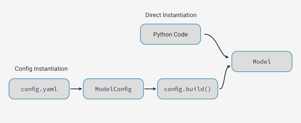
This can of course be done from code. For instance, to create a simplified model for stability analysis and a full model for nonlinear simulation we could do the following:

stability_model = SubsonicF16(
    engine=TabulatedEngine(),
    elevator=IdealActuator(),
    aileron=IdealActuator(),
    rudder=IdealActuator(),
    xcg=0.3,
)

full_model = SubsonicF16(
    engine=NASAEngine(),
    elevator=LagActuator(
        tau=0.0495,
        rate_limit=60.0,
        pos_limits=(-25.0, 25.0),
    )
    aileron=LagActuator(
        tau=0.0495,
        rate_limit=80.0,
        pos_limits=(-21.5, 21.5),
    )
    rudder=LagActuator(
        tau=0.0495,
        rate_limit=120.0,
        pos_limits=(-30.0, 30.0),
    )
)

This is perfectly fine, but becomes cumbersome as the complexity and configurability of the models grows.

Archimedes also provides capabilities for defining configuration management systems that work well with the struct-based hierarchical modeling. We won’t go into depth about how to set this up here - see the Hierarchical Modeling tutorial for details - but this allows you to define the configuration in a YAML or JSON file.

For instance, the same configurations as above can be created with the following YAML config:

stability:
  xcg: 0.3
  engine:
    type: tabulated
  elevator:
    type: ideal
  aileron:
    type: ideal
  rudder:
    type: ideal

full:
  xcg: 0.3
  atmosphere:
    type: ussa1976
  engine:
    type: nasa
  elevator:
    type: lag
    tau: 0.0495  # s
    rate_limit: 60.0  # deg/s
    pos_limits: [-25.0, 25.0]  # deg
  aileron:
    type: lag
    tau: 0.0495  # s
    rate_limit: 80.0  # deg/s
    pos_limits: [-21.5, 21.5]  # deg
  rudder:
    type: lag
    tau: 0.0495  # s
    rate_limit: 120.0  # deg/s
    pos_limits: [-30.0, 30.0]  # deg

This can be loaded and converted to models with:

from f16 import SubsonicF16

stability_model = SubsonicF16.from_yaml("config.yaml", "stability")
pprint(stability_model)

full_model = SubsonicF16.from_yaml("config.yaml", "full")
pprint(full_model)

This lets you set up several pre-baked vehicle configurations for different purposes that can be version-controlled and reused across different analysis codes.

../../_images/config_lifecycle_light.png

However, as with the hierarchical design itself, for your own use cases you may find the configuration management system to be either helpful and scalable, or complicated overkill - in either case you are probably correct.

Conclusion¶

We now have a modular, hierarchical model of F-16 flight dynamics, with components for gravity, atmosphere, aerodynamics, propulsion, and control surface actuators. We can construct the model either directly in Python, or using the configuration management system.

In the end we have SubsonicF16.dynamics(t, x, u), which computes the time derivatives given state and input data. In other words, we have gone the long way around to the same destination as the ported Fortran code in Part 1 - a nonlinear state-space model of the form:

\[\dot{x} = f(t, x, u)\]

In Part 3 we will continue on with trim and stability analysis of this model.