Subsonic F-16
In the late 1970’s NASA released detailed aerodynamic models for an F-16 based on subscale and subsonic wind-tunnel testing, along with a simplified model of the turbofan engine (Nguyen, et al., 1979). This remains an excellent benchmark for validation and development of flight control frameworks, since it is still one of the more comprehensive publicly available characterizations of a high-performance military aircraft (and the F-16 is still a workhorse today!). It is also one of the main running examples in the classic introductory GNC textbook “Aircraft Control and Simulation” by Stevens, Lewis, and Johnson, making it a great educational example as well.
In this series we’ll go through two different approaches to implementing the F-16 model. We’ll assume you are familiar with the basic principles and terminology of flight dynamics modeling; if not, the textbook above is a great place to start.
First, we’ll show essentially a direct port of the original Fortran code from Stevens, Lewis, and Johnson to Python. For existing codes in Fortran, MATLAB, etc. this is a quick and easy way to get your model working, though it does not take advantage of the hierarchical modeling or spatial mechanics capabilities in Archimedes.
Second, we’ll rewrite the same model using a hierarchical component-based approach and the RigidBody 6dof dynamics model.
This takes a little more organizational effort up front - you have to decide what your subsystems are and define clear interfaces for each of them - but the payoff is improved clarity and maintainability in the long term.
Steady turn maneuver
To skip ahead a bit, the flight dynamics model we’re building can be easily loaded, trimmed, and simulated with the same hierarchical modeling and ODE solving machinery used everywhere else in Archimedes.
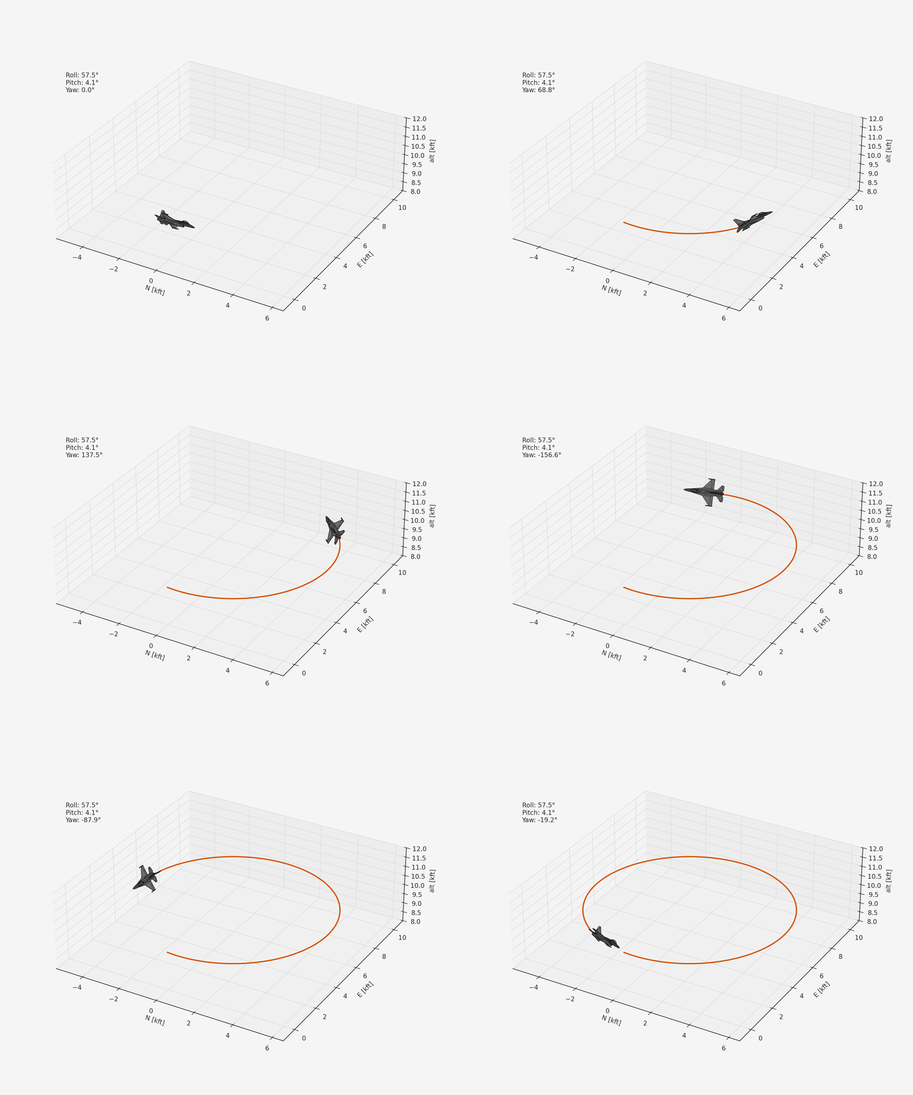
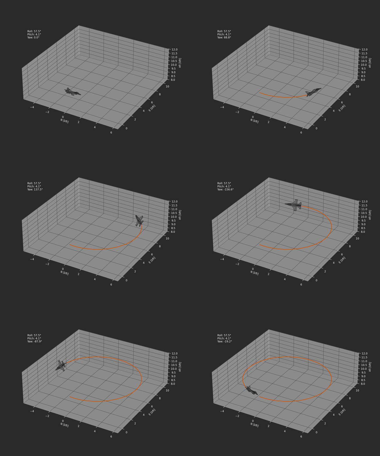
For example, here we’ll set up the F-16 with its center of gravity in a stable position and find a trimmed turning maneuver at 0.1 rad/s and 500 ft/s:
# Trim for steady level turn
model = SubsonicF16.from_yaml("config.yaml", "full")
result = model.trim(vt=500.0, turn_rate=0.1, alt=10000.0, gamma=0.0)
pprint(result.variables)
pprint(result.state)
pprint(result.inputs)
Then we can simulate the nonlinear model in the trimmed state:
x0 = result.state
u0 = result.inputs

# Flatten nested struct -> flat array for scipy
x0_flat, unravel = arc.tree.ravel(x0)


def ode_rhs(t, x_flat):
    x = unravel(x_flat)
    x_t = model.dynamics(t, x, u0)
    x_t_flat, _ = arc.tree.ravel(x_t)
    return x_t_flat


t0, tf = 0.0, 60.0
ts = np.arange(t0, tf, 0.1)
xs_flat = arc.odeint(ode_rhs, (t0, tf), x0_flat, t_eval=ts)
xs = arc.vmap(unravel)(xs_flat.T)
Note
If arc.tree.ravel and arc.vmap are not familiar, check out the documentation page on Structured Data Types.
After some matplotlib animation code and downloading a free low-poly F-16 mesh, we can visualize the trajectory:


Outline
Porting Legacy Code [OPTIONAL]
Translating the Fortran code to Archimedes
Pros and cons of the “monolithic” approach
-
Breaking down the subsystems
Implementing with
@structmodules
-
Defining dynamic trim conditions
Trimming for altitude hold, steady climb, and coordinated turns
Model decomposition
Linear stability analysis
-
Reusable flight dynamics codes
Reflections on hierarchical design patterns
Automatic differentiation
Where to go next
Prerequisites
Besides familiarity with flight dynamics, this series assumes you are familiar with the basics of Archimedes (for instance the content on the Getting Started page) and the concept of structured data types.
The code itself uses the interpolant functionality heavily for aerodynamic and propulsion lookup tables, but is otherwise plain NumPy.