Hierarchical Design Patterns
Part 1 of this tutorial covers best practices and design patterns for creating composable dynamical systems models, control algorithms, and other modular functionality using Archimedes.
By leveraging the struct decorator, you can create modular components that can be combined into complex hierarchical models while maintaining clean, organized code.
But while this guide provides some tips and best practices, these are strictly suggestions; you can design your models and workflows however you wish.
Core Concepts
The basic concepts of structured data types and tree operations are covered in the “Structured Data Types” documentation page. Here we’ll build on these concepts to see how they can be used for intuitive and scalable design patterns.
Dynamical systems often have natural subsystems and state variables that benefit from logical grouping. Using tree-structured representations allows you to:
Group related state variables together
Create nested hierarchies that mirror the physical structure of your system
Maintain clean interfaces between subsystems
Flatten and unflatten states automatically for simulation, optimization, stability analysis, etc.
Design Patterns
The first step in creating a hierarchical dynamics model is to identify the subsystems, components, etc. that naturally decompose a complex system into its logical building blocks. For each of these modular dynamics components, you can then implement state-space systems of the form
where \(t\) is time, \(x\) is the state, \(u\) are external (control) inputs, and \(p\) are parameters. Some recommended patterns to implement these components include:
Structured Data Classes: Decorate each class as a
structNested Struct Definitions: Define a
Stateclass inside each model component (andInputandOutputas necessary)Hierarchical Parameters: Add model parameters as fields in the struct or as a nested
ParametersclassStandardized Methods: Implement
dynamics(self, t, state, ...)methods that return state derivatives, and/oroutput(self, t, state, ...)methods that return the outputs of a state-space model
A template for a generic dynamics model following these patterns would look like this:
@struct
class Component:
    # Define model parameters here
    ...

    # OR create an inner struct to organize them
    @struct
    class Parameters:
        ...  # Model parameters (p)

    @struct
    class State:
        ...  # Dynamic state (x)

    @struct
    class Input:
        ...  # Inputs to the system (u)

    @struct
    class Output:
        ...  # Measured outputs (y)

    def dynamics(self, t: float, x: State, u: Input, p: Parameters) -> State:
        ...  # Implement ẋ = f(t, x, u, p)

    def output(self, t: float, x: State, u: Input, p: Parameters) -> Output:
        ...  # Implement y = h(t, x, u, p)
One important recommendation is to use abc metaclasses or Protocol classes to clearly define interfaces for components - then you can define multiple variants and easily switch between them without touching the rest of your system model.
This template code itself could be a Protocol, for instance.
Then you can create composite models by nesting these components together to organize and abstract the details of complex system models.
The abc/Protocol approach also lets you define an interface for a component and then implement “multi-fidelity modeling” by creating implementations of varying speed and accuracy.
For example, you might create a sensor component and then have three variants that implement a (1) simplified version with no dynamics, (2) a simple linear system model (e.g. second-order transfer function), and (3) a high-fidelity physics-based model. Then you can separately calibrate each using parameter estimation and easily switch between them depending on the context (e.g. low-fidelity for model-based control or high-fidelity for simulated evaluation).
We’ll see more on implementing the Protocol concept in Part 2, covering configuration management for hierarchical models.
Basic Component Pattern
Here’s a basic example of using these patterns to creating a modular dynamical system component:
@struct
class Oscillator:
    """A basic mass-spring-damper component."""

    # Define model parameters as fields in the struct
    m: float  # Mass
    k: float  # Spring constant
    b: float  # Damping constant

    # Define a nested State class as another struct
    @struct
    class State:
        """State variables for the mass-spring-damper system."""

        x: float
        v: float

    def dynamics(self, t, state: State, f_ext: float = 0.0) -> State:
        """Compute the time derivatives of the state variables."""

        # Compute derivatives
        f_net = f_ext - self.k * state.x - self.b * state.v

        # Return state derivatives in the same structure
        return self.State(
            x=state.v,
            v=f_net / self.m,
        )


system = Oscillator(m=1.0, k=1.0, b=0.1)
x0 = system.State(x=1.0, v=0.0)
x0
Oscillator.State(x=1.0, v=0.0)
Note that since this particular system is very simple we didn’t implement the full machinery shown in the Component protocol above - that would be overkill here.
In fact, for such a simple system, the advantages to following this design pattern are relatively limited overall (it would have been easier to just implement a simple ODE right-hand-side function).
But because these nodes can be nested within each other, it can be a useful way to organize states, parameters, and functions associated with more complex models.
Working with tree-structured data
Many functions like ODE solvers expect to work with flat vectors. Tree operations in Archimedes make conversion to and from flat vectors easy. For example, we can “ravel” a tree-structured state to a vector and “unravel” back to the original state:
x0_flat, unravel = arc.tree.ravel(x0)
print(x0_flat)
print(unravel(x0_flat))
[1. 0.]
Oscillator.State(x=array(1.), v=array(0.))
The unravel function created by tree.ravel is specific to the original argument data type, so it can be used within ODE functions, for example:
@arc.compile
def ode_rhs(t, state_flat, system):
    # Unflatten the state vector to our structured state
    state = unravel(state_flat)

    # Compute state derivatives using model dynamics
    state_deriv = system.dynamics(t, state)

    # Flatten derivatives back to a vector
    state_deriv_flat, _ = arc.tree.ravel(state_deriv)

    return state_deriv_flat


# Solve the ODE
t_span = (0.0, 10.0)
t_eval = np.linspace(*t_span, 100)
solution_flat = arc.odeint(
    ode_rhs,
    t_span=t_span,
    x0=x0_flat,
    t_eval=t_eval,
    args=(system,),
)
Since the model itself is also a struct, we can also apply ravel directly to it, giving us a flat vector of the parameters defined as fields:
p_flat, unravel_system = arc.tree.ravel(system)
print(p_flat)  # [1.  1.  0.1]
[1. 1. 0.1]
This is useful for applications in optimization and parameter estimation.
Another common pattern is to define yet another struct for the parameters, rather than having them as fields in the system model.
This comes down to individual preference and whatever works best for the specific application.
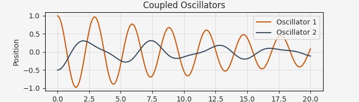
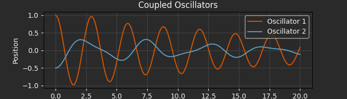
Composite System: Coupled Oscillators
Larger systems can be built by composing multiple components together:
@struct
class CoupledOscillators:
    """A system of two coupled oscillators."""

    osc1: Oscillator
    osc2: Oscillator
    coupling: float

    @struct
    class State:
        """Combined state of both oscillators."""

        osc1: Oscillator.State
        osc2: Oscillator.State

    def dynamics(self, t, state):
        """Compute dynamics of the coupled system."""
        # Extract states
        x1 = state.osc1.x
        x2 = state.osc2.x

        # Compute equal and opposite coupling force
        f_ext = self.coupling * (x2 - x1)

        return self.State(
            osc1=self.osc1.dynamics(t, state.osc1, f_ext),
            osc2=self.osc2.dynamics(t, state.osc2, -f_ext),
        )


# Create a coupled oscillator system
system = CoupledOscillators(
    osc1=Oscillator(m=1.0, k=4.0, b=0.1),
    osc2=Oscillator(m=1.5, k=2.0, b=0.2),
    coupling=0.5,
)

# Create initial state
x0 = system.State(
    osc1=Oscillator.State(x=1.0, v=0.0),
    osc2=Oscillator.State(x=-0.5, v=0.0),
)

# Flatten the state for ODE solver
x0_flat, state_unravel = arc.tree.ravel(x0)


# ODE function that works with flat arrays
@arc.compile
def ode_rhs(t, state_flat, system):
    state = state_unravel(state_flat)
    state_deriv = system.dynamics(t, state)
    state_deriv_flat, _ = arc.tree.ravel(state_deriv)
    return state_deriv_flat


# Solve the system
t_span = (0.0, 20.0)
t_eval = np.linspace(*t_span, 200)
sol_flat = arc.odeint(
    ode_rhs,
    t_span=t_span,
    x0=x0_flat,
    t_eval=t_eval,
    args=(system,),
)

# Postprocessing: create a "vectorized map" of the unravel
# function to map back to the original tree-structured state
sol = arc.vmap(state_unravel, in_axes=1)(sol_flat)
[Advanced]: Derived Quantities
One situation that commonly arises in complex systems are intermediate values that are reused in multiple places and are relatively expensive to compute. For example, the dynamic pressure and Mach number calculation in flight dynamics requires querying an atmosphere model, and these quantities are often used by both the aerodynamic and propulsion subsystems. This also comes up when modeling thermal fluids, where an equation of state model is used to calculate various thermodynamic properties based on primitive state variables, and these derived properties might be re-used in several places.
These derived quantities are not part of the dynamic state, and so the obvious solutions are:
Recalculate the derived values anywhere they’re needed
Calculate once and pass as arguments to other functions/subsystems
The first option is obviously not ideal, since it requires duplicate computation. The second choice is workable, but requires manually keeping track of all such derived quantities.
You can handle this situation in several ways, but one relatively clean approach is to create an extra struct to hold all of these, and then pass the entire container around as needed.
For example, in the Subsonic F-16 example, the derived quantities are kept in a FlightCondition struct.
It works something like this:
@struct
class FlightCondition:
    alt: float  # Altitude
    vt: float  # True airspeed
    alpha: float  # Angle of attack
    beta: float  # Sideslip angle
    mach: float  # Mach number
    qbar: float  # Dynamic pressure


@struct
class SubsonicF16:

    @struct
    class State(RigidBody.State):
        ...

    @struct
    class Input:
        ...

    def flight_condition(self, x: RigidBody.State) -> FlightCondition:
        ...  # Compute TAS, AoA, etc.

    def net_forces(
        self, t, x: State, u: Input, condition: FlightCondition | None = None
    ) -> tuple[np.ndarray, np.ndarray]:
        """Calculate forces and moments in body frame"""
        if condition is None:
            condition = self.flight_condition(x)

        ...

    def dynamics(self, t, x: State, u: Input) -> State:
        """Compute time derivative of the state"""
        condition = self.flight_condition(x)

        # Compute the net forces
        F_B, M_B = self.net_forces(t, x, u, condition)

        ...
This works well because it’s scalable to any amount of derived data without changing the function interfaces.
It also provides a pattern where methods like net_forces can be called for offline analysis without calculating the derived quantities, but for simulation or other “online” work there’s no duplicate calculation.
This situation doesn’t come up in every model, so there’s no need to shoehorn this pattern in where it doesn’t belong. But keep it in mind as a convenient way to handle this kind of intermediate “derived” data.
Summary
The recommended approach to building hierarchical and modular dynamical systems in Archimedes follows these key patterns:
Use
@structto define structured component classesCreate nested
Stateclasses to organize state variables (and maybeInput,Output,Parameters)Implement
dynamicsmethods that compute state derivatives (and maybeoutput)Compose larger systems from smaller components
Add helper methods to simplify simulation and analysis
Other best practices include:
Immutable States: Always return new state objects instead of modifying existing ones
Physical Units: Document physical units in comments or docstrings
Meaningful Names: Use descriptive names that reflect physical components, or consistent pseudo-mathematical notation like the monogram convention
Domain Decomposition: Decompose complex systems into logical components (mechanical, electrical, etc.)
Physical Parameters: Define physical parameters as fields in the structs or as inner classes
Configuration Parameters: Define as fields in the struct and use the
field(static=True)annotation.
These patterns enable clean, organized, and reusable model components by leveraging Archimedes’ tree operations to handle the conversion between structured and flat representations needed by ODE solvers.