Introducing Archimedes

A Python toolkit for deployable control systems engineering
By Jared Callaham • 6 Oct 2025
A great engineer (controls being no exception) has to be part hacker, part master craftsman.
You have to be a hacker because things rarely “just work” in the real world without a little… creativity. But you can’t only be a hacker; developing complex systems in aerospace, automotive, robotics, and similar industries demands a disciplined, systematic approach. You need tools that let you iterate fast and maintain a methodical workflow where changes are version-controlled, algorithms are tested systematically, and deployment is repeatable.
Modern deep learning frameworks solved this years ago — you can develop in PyTorch or JAX and deploy anywhere. But those tools were built for neural net models, GPUs, and cloud deployments, not dynamics models, MCUs, and HIL testing.
That’s where Archimedes comes in; what PyTorch did for ML deployment, Archimedes aims to do for control systems. The goal is to build an open-source “PyTorch for hardware” that gives you the productivity of Python with the deployability of C.
In short, Archimedes is a Python framework that lets you develop and analyze algorithms in NumPy and automatically generate optimized C code for embedded systems. For instance, you can write a physics model in Python, calibrate it with data, use the model to design and simulate control logic, validate with simple hardware-in-the-loop (HIL) testing, and deploy with confidence:
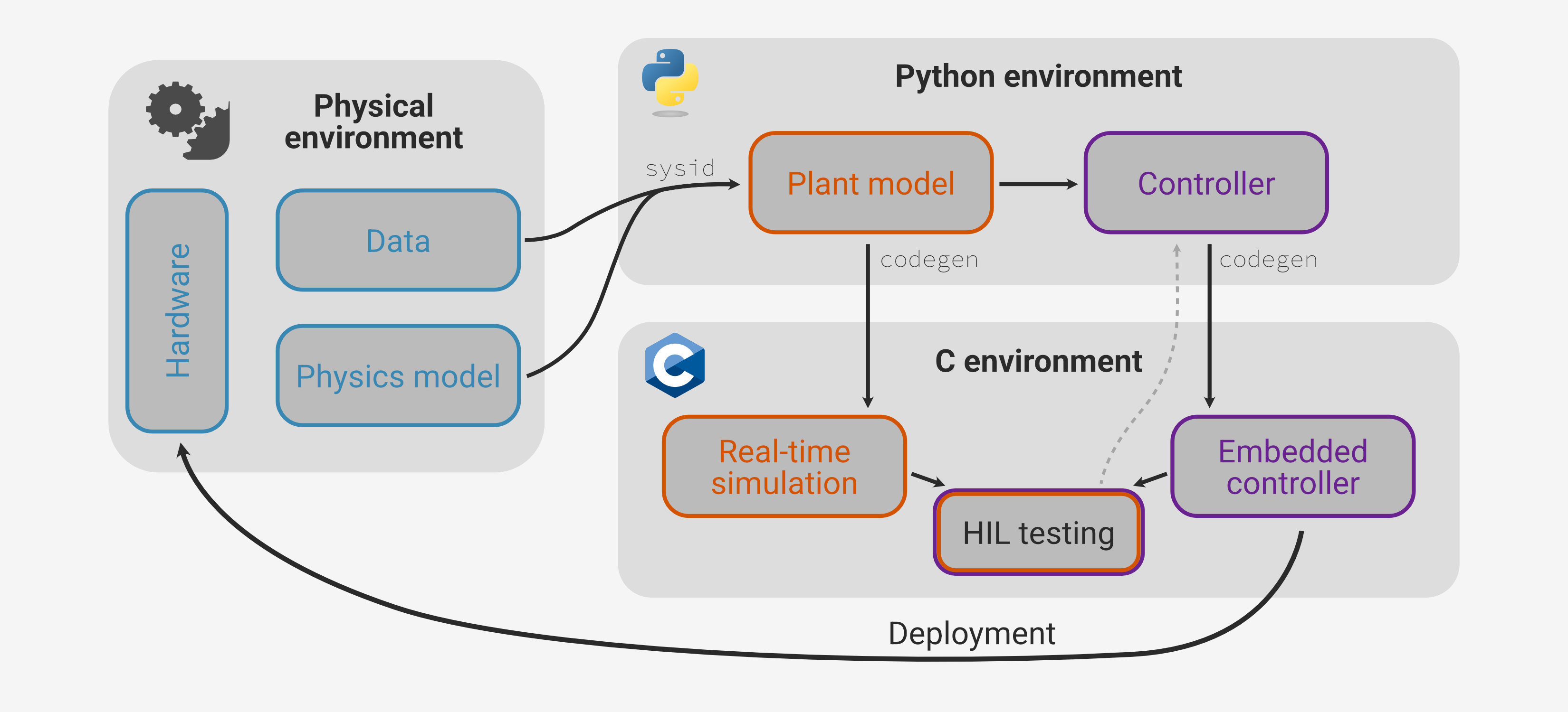
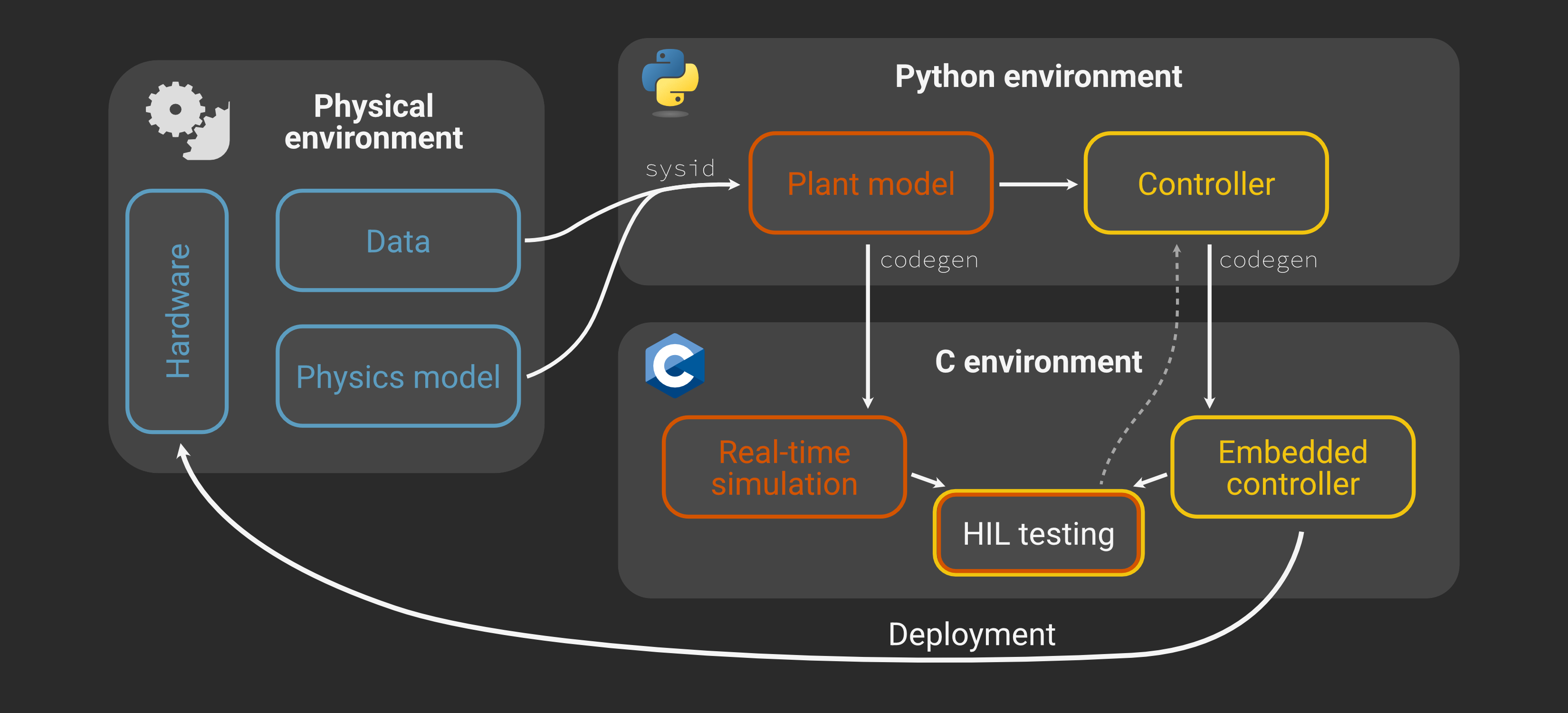
This is one workflow you might use with Archimedes (specifically, the one from the hardware deployment tutorial), but it’s designed to be flexible, so you’re free to build up whatever workflow suits your style and application best.
The Linchpin: Python → C Code Generation
Archimedes started with the question, “What would you need to actually do practical control systems development in Python?”
As a high-level language, it’s hard to beat Python on design principles like progressive disclosure, flexibility, and scalability. The numerical ecosystem (NumPy, SciPy, Matplotlib, Pandas, PyTorch, etc.) is also excellent. The problem is that none of it can deploy to typical embedded systems.
If you need to deploy to hardware today, you have a few basic options:
Work in a high-level language like Python or Julia and manually translate algorithms to C code
Work entirely in a low-level language like C/C++ or Rust
Adopt an expensive vendor-locked ecosystem that supports automatic code generation
(Side note: While running Python itself on a microcontroller is growing in popularity for educational and hobby applications, there’s no real future for pure Python in real-time mission-critical deployments.)
However, if you could do seamless C code generation from standard NumPy code, you could layer on simulation and optimization tools, building blocks for physics modeling, testing frameworks, and other features of comprehensive controls engineering toolchains. But without the code generation, there will always be a gulf between the software and the hardware deployment.
Just to drive the point home, here’s a side-by-side of manual vs automatic coding for a common piece of sensor fusion algorithms:
Kalman Filter Comparison
Below are two implementations of a Kalman filter, an algorithm that combines noisy sensor measurements with a prediction model to estimate system state. This is what’s behind GPS navigation, spacecraft guidance, and sensor fusion in millions of devices.
On the left is hand-written C code, and on the right is a NumPy version that can be used to generate an equivalent function.
Here we’ll show an implementation for the common case of a single sensor, which avoids having to use a library for matrix inversion in C (though Archimedes does support operations like Cholesky factorization).
#include <stdint.h>
#define N_STATES        4

typedef struct {
    float H[N_STATES];  // Measurement matrix (1 x n)
    float R;            // Measurement noise covariance (scalar)
} kf_params_t;

typedef struct {
    float x[N_STATES];            // State estimate
    float P[N_STATES][N_STATES]; // Estimate covariance
} kf_state_t;

typedef struct {
    float K[N_STATES];              // Kalman gain (n x 1)
    float M[N_STATES][N_STATES];    // I - K * H temporary
    float MP[N_STATES][N_STATES];   // M * P temporary
    float MPMT[N_STATES][N_STATES]; // M * P * M^T temporary
    float KRKT[N_STATES][N_STATES]; // K * R * K^T temporary
} kf_work_t;

/**
 * Kalman filter update step (scalar measurement case)
 *
 * Mathematical formulation:
 *   y = z - H·x                      (innovation)
 *   S = H·P·H^T + R                  (innovation covariance)
 *   K = P·H^T·S^(-1)                 (Kalman gain)
 *   x' = x + K·y                     (state update)
 *   P' = (I-KH)·P·(I-KH)^T + K·R·K^T (Joseph form covariance)
 *
 * @param z: Latest measurement
 * @param kf_state: Pointer to Kalman filter state struct
 * @param kf_params: Pointer to Kalman filter parameters struct
 * @param kf_work: Pointer to Kalman filter work struct (for temporaries)
 * @return: 0 on success, -1 on error
 */
int kalman_update(float z, kf_state_t *kf_state,
                  const kf_params_t *kf_params,
                  kf_work_t *kf_work) {
    #ifdef DEBUG
    if (!kf_state || !kf_params || !kf_work)
        return -1;
    #endif
    size_t i, j, k;

    // Innovation: y = z - H * x
    float y = z;
    for (i = 0; i < N_STATES; i++)
        y -= kf_params->H[i] * kf_state->x[i];

    // Innovation covariance: S = H * P * H^T + R
    float S = kf_params->R;

    // Compute P * H^T (mv_mult)
    // Using K as temporary storage here
    for (i = 0; i < N_STATES; i++) {
        kf_work->K[i] = 0.0f;
        for (j = 0; j < N_STATES; j++) {
            kf_work->K[i] += kf_state->P[i][j] * kf_params->H[j];
        }
    }
    for (i = 0; i < N_STATES; i++)
        S += kf_params->H[i] * kf_work->K[i];

    // Kalman gain: K = P * H^T / S
    for (i = 0; i < N_STATES; i++)
        kf_work->K[i] /= S;

    // Update state with feedback from new measurement: x = x + K * y
    for (i = 0; i < N_STATES; i++)
        kf_state->x[i] += kf_work->K[i] * y;

    // Joseph form update: P = (I - K * H) * P * (I - K * H)^T + K * R * K^T
    // First compute M = I - K * H
    for (i = 0; i < N_STATES; i++) {
        for (j = 0; j < N_STATES; j++) {
            if (i == j)
                kf_work->M[i][j] = 1.0f - kf_work->K[i] * kf_params->H[j];
            else
                kf_work->M[i][j] = -kf_work->K[i] * kf_params->H[j];
        }
    }

    // Compute M * P
    for (i = 0; i < N_STATES; i++) {
        for (j = 0; j < N_STATES; j++) {
            kf_work->MP[i][j] = 0.0f;
            for (k = 0; k < N_STATES; k++) {
                kf_work->MP[i][j] += kf_work->M[i][k] * kf_state->P[k][j];
            }
        }
    }

    // Compute (M * P) * M^T
    for (i = 0; i < N_STATES; i++) {
        for (j = 0; j < N_STATES; j++) {
            kf_work->MPMT[i][j] = 0.0f;
            for (k = 0; k < N_STATES; k++) {
                kf_work->MPMT[i][j] += kf_work->MP[i][k] * kf_work->M[j][k];
            }
        }
    }

    // Compute K * R * K^T
    for (i = 0; i < N_STATES; i++) {
        for (j = 0; j < N_STATES; j++) {
            kf_work->KRKT[i][j] = kf_work->K[i] * kf_params->R * kf_work->K[j];
        }
    }

    // Final covariance update: P = MPMT + KRKT
    for (i = 0; i < N_STATES; i++) {
        for (j = 0; j < N_STATES; j++) {
            kf_state->P[i][j] = kf_work->MPMT[i][j] + kf_work->KRKT[i][j];
        }
    }

    return 0;
}
@arc.compile
def kalman_update(x, P, z, H, R):
    """Update state estimate with new measurement"""
    I = np.eye(len(x))
    R = np.atleast_2d(R)  # Ensure R is 2D for matrix operations

    y = np.atleast_1d(z - H @ x)  # Innovation
    S = H @ P @ H.T + R  # Innovation covariance
    K = P @ H.T / S  # Kalman gain (scalar S)

    # Update state with feedback from new measurement
    x_new = x + K * y

    # Joseph form covariance update
    P_new = (I - K @ H) @ P @ (I - K @ H).T + K @ R @ K.T

    return x_new, P_new

# Generate optimized C code:
return_names = ("x_new", "P_new")
args = (x, P, z, H, R)
arc.codegen(kalman_update, args, return_names=return_names)
Neither of these implementations is optimized, but it gives a sense of what it looks like to work in either environment. Of course, for production hand-written code, you’d likely also use optimized linear algebra libraries like CMSIS-DSP and numerical strategies like Cholesky factorization or a square-root form for stability. But the extra numerical features are only a few extra lines in NumPy, while the hand-written C version becomes more and more complex.
This capability, and most of the other core functionality in Archimedes, is made possible by building on CasADi, a sophisticated open-source library for nonlinear optimization and algorithmic differentiation. This lets Archimedes translate your NumPy code into C++ computational graphs that support code generation, derivative calculation, and more.
Beyond Codegen
If you’re already working in C/C++/Rust, or if you don’t actually need to deploy to hardware for your application, the codegen may not speak to you. But while Python → C code generation is what makes Archimedes practical for deployment, there’s much more you can do.
Compilation
Archimedes can “compile” a Python function into a C++ computational graph, meaning that when you call the compiled function, the entire numerical code gets executed in C++ rather than interpreted Python. For complicated functions this can achieve dramatic speedups over pure Python (5-10x even on simple benchmarks).
import numpy as np
import archimedes as arc

@arc.compile
def rotate(x, theta):
    R = np.array([
        [np.cos(theta), -np.sin(theta)],
        [np.sin(theta), np.cos(theta)],
    ], like=x)
    return R @ x

rotate(np.array([1.0, 0.0]), 0.1)
You can embed complex functionality like ODE solves, constrained nonlinear optimization, and more directly in these computational graphs.
When you first call your function, Archimedes feeds it symbolic arrays (using CasADi’s symbolic types under the hood) that match the shape and type of your numerical inputs. As your code executes, it builds up a C++ representation of the calculation. Then, instead of operating on the numerical arrays, your code operates on these symbolic replacements, using NumPy’s array dispatch mechanism to redirect to CasADi whenever you call NumPy functions. By the end of this “tracing” step, CasADi has a full view of what the function does and can reproduce it in efficient C++. Then, any time you call that function again, the C++ equivalent is what actually gets executed.
This approach is not “Just-In-Time” (JIT) compilation in the sense used by Julia/JAX/Numba, where the Python code is literally compiled down to highly optimized platform-specific machine code. We’ll show some benchmarking in a separate post, but generally what you can expect is that these JIT-compiled frameworks will be somewhat faster than pre-compiled CasADi (and hence, Archimedes). However, by avoiding the overhead and “unrolling” of true JIT compilation, we get a massive reduction in compilation time for the kind of complex functions typical of advanced controls applications.
For more on how this works (and when it doesn’t), see the Under the Hood documentation page.
Simulation, Optimization, & Root-finding
Archimedes provides a SciPy-like interface to the powerful and robust CVODES solver from SUNDIALS, which is a highly efficient and time-tested implementation of a stiff/non-stiff implicit solver that even supports gradient-based sensitivity analysis:
def simulate(x0):
    xs = arc.odeint(dynamics, (t0, tf), x0, t_eval=ts)
    return xs[:, -1]

arc.jac(simulate)(x0)  # dxf/dx0
We also have a SciPy-like optimization interface that can solve constrained nonlinear problems with IPOPT:
# Rosenbrock problem
def f(x):
    return 100 * (x[1] - x[0] ** 2) ** 2 + (1 - x[0]) ** 2

result = arc.minimize(f, x0=[-1.0, 1.0])
and a root-finding interface for iteratively solving nonlinear algebraic systems using Newton iterations and similar methods:
def f(x):
    return np.array([
        x[0] + 0.5 * (x[0] - x[1])**3 - 1.0,
        0.5 * (x[1] - x[0])**3 + x[1]
    ], like=x)

x = arc.root(f, x0=np.array([0.0, 0.0]))
These solves can also be embedded in compiled computational graphs for accelerated simulation and optimization.
Automatic Differentiation
Compilation into a CasADi computational graph unlocks two critical capabilities: execution speed and automatic differentiation. This means that you can easily and accurately calculate derivatives of your functions:
def lotka_volterra(t, x):
    a, b, c, d = 1.5, 1.0, 1.0, 3.0
    return np.hstack([
        a * x[0] - b * x[0] * x[1],
        c * x[0] * x[1] - d * x[1],
    ])

# Linearize the system
J = arc.jac(dynamics, argnums=1)
print(J(0.0, [1.0, 1.0]))
Besides linearizing models for stability analysis and controller design, this is a feature you may not directly use very often. But gradients and Jacobians are used pervasively in numerical methods:
Optimization solvers use gradients of the objective, Jacobians of the constraints, and sometimes even Hessian information
Simulation algorithms use Jacobians of the dynamics model for implicit solvers, especially for “stiff” ODE/DAE problems
Root-finding solvers like Newton’s method use Jacobians at every iteration to find an improved guess at the solution point
So when you do parameter estimation, trajectory optimization, trim point identification, or even just call odeint, you don’t think about “autodiff”, but it’s happening behind the scenes to solve your problem.
Traditional scientific computing packages like SciPy and MATLAB usually fall back to slow and inaccurate finite differencing unless you provide manually implemented gradients, Jacobians, etc. - but for anything but the simplest problems this is prohibitively complicated to calculate and implement.
Newer frameworks like Julia, JAX, and PyTorch rely much more heavily on autodiff, but none of these are tailored towards hardware and controls engineering applications. My personal experience has been that CasADi (the autodiff framework used under the hood by Archimedes) has far and away the best autodiff system for the kinds of large, sparse problems that commonly arise in engineering (like parameter estimation, trajectory optimization, model-predictive control, etc.).
All that is to say, the derivatives are there if you need them.
Structured Data Types
Most numerical codes are naturally written to operate on flat vectors. This makes sense for the implementation of an optimization algorithm or ODE solver, but physical systems are usually more naturally conceived of as hierarchical. For instance, a satellite has position, velocity, attitude, angular velocity, battery state, thermal state, etc. To work with typical numerical codes, you have to either keep track of what entries in your array are which physical state or manually flatten/unflatten every time you call a routine that expects a flat vector.
That might be fine the first time, but what if you want to try a higher-fidelity battery model that has twice as many dynamic states? It quickly becomes a nightmare to maintain these kinds of codes, and the result is that you waste cycles on keeping all of this straight, and you lose the practical capability to explore multi-fidelity modeling.
This also comes up frequently in deep learning: models are naturally organized as hierarchical modules with trainable parameters.
This is the root of the nn.Module in PyTorch and the “PyTree” concept in JAX.
Modern ML frameworks (specifically JAX and PyTorch) have developed a nice set of solutions around working with this kind of hierarchically structured data.
But this hierarchical data and logic might even be more common in engineering. Physical systems are naturally organized into subsystems and components that have well-defined interfaces, and each of these might have its own dynamic state and configurable parameters. Hierarchical data structures can mirror this physical system decomposition.
Archimedes takes inspiration from these frameworks and supports “tree operations” (functions applied to hierarchical data) and a @struct decorator to create tree-compatible data classes:
@arc.struct
class PointMass:
    pos: np.ndarray
    vel: np.ndarray

state = PointMass(np.zeros(3), np.ones(3))  # state.pos, state.vel
flat_state, unravel = arc.tree.ravel(state)  # flat_state is a vector
state = unravel(flat_state)  # Back to a PointMass instance
These @struct-decorated classes can be nested inside one another, flattened to/from a 1D vector, and used to auto-generate nested struct types in deployable C code.
If a PointMass is used as an argument to a codegen function, it will become:
typedef struct {
    float pos[3];
    float vel[3];
} point_mass_t;
This gives you a predictable and intuitive way to switch back and forth between Python and auto-generated C.
For much more on structured data types, see Structured Data Types, Hierarchical Systems Modeling, and the C Code Generation tutorial series.
Why Another Framework?
There are lots of modeling and simulation tools out there, from rock-solid commercial tools building on 30-year legacies to innovative modern frameworks experimenting with new languages, JIT-compilation, and physics-informed ML.
I created Archimedes because none of these really solved the problems I was having in my own work. Codebases that started out being logical and well-organized invariably ended up growing into a gnarled, difficult-to-maintain mass in order to support increasingly complex models and analyses. Then when it’s time to move towards testing and production, you’re back to square one to translate to C code.
Granted, these complaints might just indicate that I’m not a great software developer - but I’m not a software developer. That’s the point. I wanted a framework that would let me write code that looked as clean as a deep learning repository in PyTorch, but would also be high-performance for simulation and optimization, and had a path to hardware deployment. After seeing it perform in my own work, I’m convinced this approach - NumPy-based development with automatic C deployment - could help how control systems engineers develop and deploy algorithms.
One last comment: from personal experience, it takes a little time (but maybe less than you think) to grok the functional programming and hierarchical data types that are core to Archimedes. (I’ve spent a lot of time in JAX, which heavily influenced the design of this library.) It’s different than what you might be used to, and there are also some quirks and gotchas related to compilation and control flow.
But these concepts do actually map quite neatly to our mental/mathematical models for dynamical systems and control algorithms. Once it clicks, you’ll be able to write clean, modular, maintainable workflows that cut down your iteration time and make it faster to design, debug, deploy, and debug, and debug, and redesign, and debug, and…
Get Started
If you want to give Archimedes a try, it’s easy to get started. The Quickstart page will walk you through the setup, and Getting Started will teach you the basic concepts.
Then there are tutorials and deep dives on:
The Hardware Deployment tutorial is a bit more advanced, but shows an end-to-end example of the kinds of workflows you can build in Archimedes.
Upcoming tutorial and example content includes 6dof flight vehicle dynamics, rotor aerodynamics, system identification, low-cost HIL testing workflows, and deep dives on C code generation.
To see where the project is headed and some more detail on the vision, also check out the roadmap.
On-ramp Projects
Once you learn the basics, I bet in an hour or two you could:
Deploy a PI temperature controller to an Arduino
Write an integrator for the IMU strapdown equations
Run parameter estimation on some step response data you have lying around
Design an energy-shaping controller for a pendulum
Benchmark some old hand-written C code against the auto-generated equivalent (and share the results)
If you have a cool first project that you’re willing to share, feel free to post about it on the Discussions page - if it’s interesting it could become its own tutorial or blog post.
“Public Beta” Status
This post marks the release of Archimedes in “public beta” (v0.X.X). This means that the core functionality is there and has already been tested in practical applications. The API is also well-tested and stable; while it is likely to evolve in time, it will change with semantic versioning conventions, meaning smooth upgrade paths and deprecation notices. The library will remain in beta for 6-12 months to allow for community feedback and API maturation across ongoing real-world applications.
For symbolic/numeric reliability in particular, Archimedes gets a big leg up by using CasADi as its backend, which has an excellent track record and is widely and actively used and tested in a variety of applications.
All that is to say, between now and the “v1.0” release you can expect things to be largely stable, but this additional time builds in a cushion to work out any kinks.
Ongoing development priorities are outlined in detail in the roadmap, but key focus areas include:
Hybrid Simulations: Support for DAEs, zero-crossing events, multirate control logic
Hardware Deployment: Improved support for HIL testing, static analysis, and profiling/telemetry
Physics Modeling: Built-in functionality like reference frames, kinematic trees, polynomial/spline primitives, and templates for domain-specific components.
Algorithm Development: State machines, trajectory optimization, MPC, sensor fusion, uncertainty quantification, etc.
Stay Updated
For updates on Archimedes, including release announcements, new features, blog posts, application examples, and case studies, subscribe to the free newsletter:
You can expect infrequent posts (maybe monthly) with a strong technical focus - no ads, spam, or paywalls.
Supporting Archimedes
This post might read a bit like ad copy, but Archimedes is a free, open-source project. The codebase, ongoing status, and discussions all live on the GitHub repository.
If you want to support it, the best thing you can do right now is try it out and give feedback. What worked well? What didn’t work? What did you like? What was confusing? What was confusing at first but you liked once you got used to it? What would you like to try with Archimedes? What would you like to try but there’s a functionality gap?
The Discussions page is a great place to share general feedback, and bug reports or feature requests are welcome on the Issues tab.
Besides feedback, other easy ways to support the project include:
⭐ Star the Repository: This shows support and interest and helps others discover the project
📢 Spread the Word: Think anyone you know might be interested?
🐛 Report Issues: Detailed bug reports, documentation gaps, and feature requests are invaluable
🗞️ Stay in the Loop: Subscribe to the newsletter for updates and announcements
Thanks for checking out the project!