Parameter Estimation for a Li-ion Battery Cell
Equivalent circuit modeling with Archimedes
Jared Callaham • 20 Mar 2026
Lithium-ion batteries are everywhere today, part of broader efforts in electrification. One of the most important emerging battery applications is energy storage in electric vehicles (EV). Compared to typical consumer electronics battery usage, this is actually an extremely demanding environment for batteries; large and unpredictable current draws, regenerative braking, load balancing across cells, and fast charging are taxing and can quickly degrade battery health if not managed properly.
The battery management system (BMS) is the set of electronics and software that manage the state-dependent charge/discharge behavior in EV batteries. Modern BMS implementations often rely on reasonably accurate dynamics models of the batteries, at a minimum for estimating the state of charge and health of the battery cells.
Li-ion battery dynamics are governed by complex electrochemistry that can be simulated with high-fidelity finite-element physics models, but this is neither practical nor necessary for embedded BMS applications. For controls purposes Li-ion dynamics can often be modeled with simple Thevenin equivalent circuit models (ECMs). These are semi-empirical models that capture the coarse-grained dynamics (e.g. multiple relaxation timescales, over- and under-voltage), are easy to understand and analyze, and are efficient enough for real-time deployment and model-based state estimation using, for instance, extended Kalman filters.
The challenge with constructing an ECM is choosing the right circuit component parameters to match the real battery behavior over a wide range of operating conditions. In this post we’ll walk through a simple way to automate this process with parameter estimation.
For more background on Li-ion battery dynamics, Gregory Plett’s ECE 5710 course notes are an excellent overview. Parameter estimation in Archimedes is covered in a tutorial using a simple ODE model, but it’s not necessary to read the tutorial in order to follow this post.
We’ll be using real data from the University of Maryland’s CALCE dataset based on tests of an INR 18650-20R 2 Ah NMC Li-ion battery cell. To run this yourself, see the GitHub repository, which includes scripts for downloading and pre-processing the raw CALCE data.
The Equivalent Circuit Model
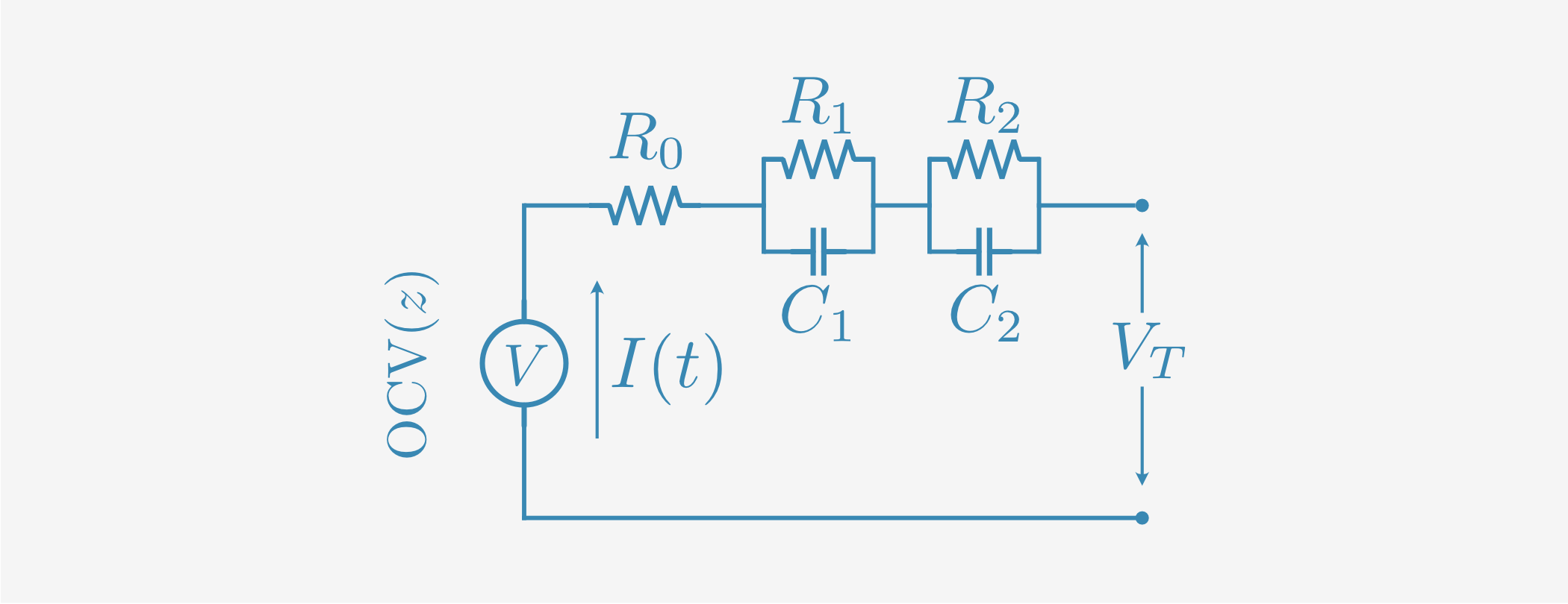

Equivalent circuit models can vary somewhat in structure, but have a common parallel-RC form. The key internal variable is the “state of charge” (SOC) \(z\), a dimensionless number ranging from 0-1 that correlates with the remaining charge in the battery. For a battery with nominal capacity \(C\) in Ah, the remaining useful energy in the battery is approximately \(zC\). This is only approximate because the nominal capacity is typically not exactly the same as the actual capacity, and the usable energy depends somewhat on the charge/discharge profile - but the SOC is an extremely useful concept even if not precisely defined.
A typical ECM consists of three kinds of components:
The open-circuit voltage (OCV): The equilibrium voltage you’d see across the terminals with zero current draw.
An inline resistor \(R_0\)
Some small number of parallel RC pairs (\(R_i\), \(C_i\))
The OCV has a characteristic dependence on the state of charge, often called the SOC-OCV curve. The other effective component values depend primarily on the SOC, with variations due to temperature, battery health degradation, and other subscale physics.
However, at constant temperature and above ~10% charge, the circuit parameters can be approximated as roughly constant. A state-space model for an \(N\)-th order ECM with current discharge \(I(t)\) is thus:
This is a single-input, single-output system with input \(I\) and measurement \(V_T\) (the battery cell terminal voltage). The state of charge \(z\) is drained directly by the current, normalized using the nominal battery capacity \(C\) in Ah (scaled to seconds for the dynamics model). Usually \(N=1\) or \(2\) RC pairs are used for typical ECMs; in this example we will use \(N=2\) for a second-order “2RC” model.
There are a couple of useful things to note about the structure of this model:
By construction, the OCV is the steady-state voltage reached after a long period with no current. So (neglecting hysteresis), the OCV-SOC curve can be measured directly using an appropriate test protocol.
Except for the OCV, which is only used in the measurement equation, this is a linear dynamical system. We won’t use this in our parameter estimation algorithms, but it’s helpful to note; because the system is linear we know exactly how it will behave for any arbitrary input profile, making “generalization to unseen data” trivial.
The dynamic response is fully characterized by \(N\) RC time constants: \(\tau_i = R_i C_i\)
Although we are assuming that the OCV only depends on \(z\) and that the \((R, C)\) values are constant, generalization to temperature-dependence and state-dependent circuit parameters is straightforward by replacing the constants with functional forms, tabulated data, or interpolants. The system remains “quasi-linear”, in the sense that you can still quantify the time constants at any operating point.
These are great properties for a data-driven model to have. The model structure (linear dynamics with a static output nonlinearity) tightly constrains its dynamic behavior and makes it highly interpretable and predictable. We can understand qualitatively what each of the parameters “means”, and we can be confident in how the model will behave when run against inputs that weren’t in the identification data set. This is a big part of why equivalent circuit models are so widely used in BMS applications.
Parameter Estimation
SOC-OCV curve
As we’ve seen, the biggest unknown in the model is the OCV-SOC curve, which can be identified directly from a properly constructed charge/discharge test. Here we’ll use the CALCE incremental current test, which proceeds as follows:
Charge the battery to 100% SOC
Discharge at C/2 current (1 Amp) until 10% of the charge is drained
Allow the cell to equilibrate
Repeat steps 2-3 until battery is fully discharged
Charge the battery to 100% in increments of 10% using steps 2-4
df = pd.read_excel("calce/12_2_2015_Incremental OCV test_SP20-1.xlsx", sheet_name="Channel_1-005_1", usecols="B,G:J")

fig, ax = plt.subplots(2, 1, figsize=(7, 4), sharex=True)
ax[0].plot(df["Test_Time(s)"], -df["Current(A)"])
ax[0].grid()
ax[0].set_ylabel("Current [A]")
ax[0].set_ylim([-0.1, 1.1])
ax[1].plot(df["Test_Time(s)"], df["Voltage(V)"])
ax[1].grid()
ax[1].set_xlabel("Time [s]")
ax[1].set_ylabel("Voltage [V]")

ax[-1].set_xlim([5000, df["Test_Time(s)"].iloc[-1]])

ax[0].set_title("Incremental Discharge Test")
plt.show()
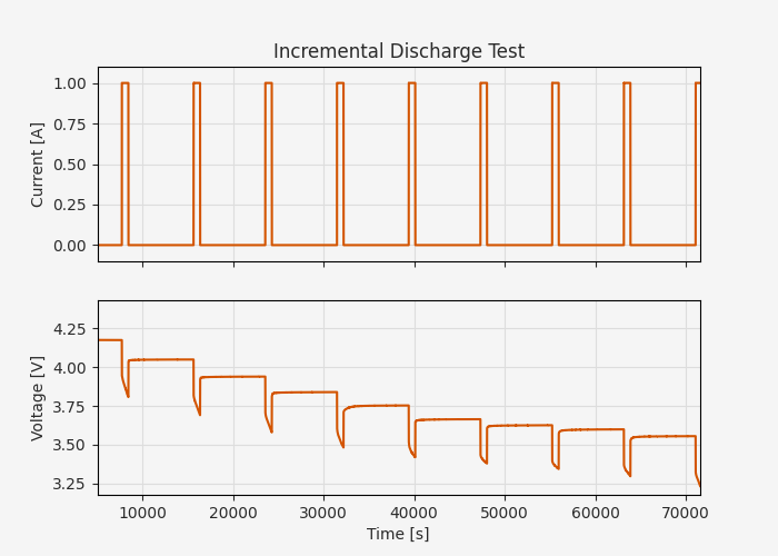
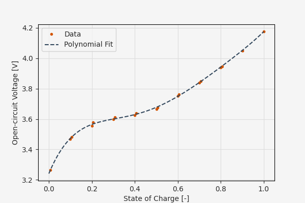
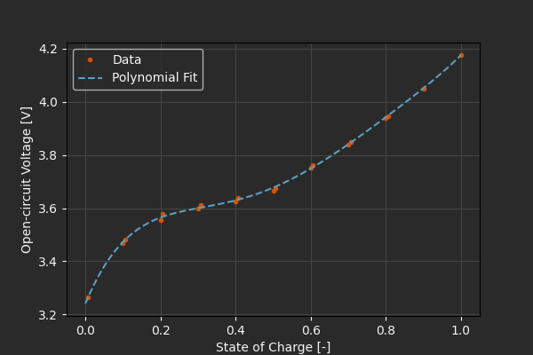
We can extract the approximate OCV values by simply looking at the final voltages prior to the next charge/discharge step. Li-ion cells can exhibit some hysteresis, so we want to do this both on the charge and discharge sides. This gives us nearly steady-state OCV values at 10% SOC increments, and we can fit a polynomial to it to get fast interpolated estimates.
Of course, in general we have to be extremely cautious about polynomial fitting, since polynomials don’t obey any kind of bounds or constraints and can oscillate wildly between data points or beyond the fitting interval. In this case, though, our domain is strictly clamped to \(z \in (0, 1)\) and we can see that a fifth-order polynomial is well-behaved and seems like a reasonable interpolant.
df = pd.read_csv("calce/SOC-OCV.csv")
soc_steady = df["SOC"].values / 100
ocv_steady = df["OCV"].values

ocv_coeffs = np.polyfit(soc_steady, ocv_steady, 5)

plt.figure(figsize=(6, 4))
plt.plot(soc_steady, ocv_steady, '.', label="Data")
soc_plt = np.linspace(0, 1, 100)
plt.plot(soc_plt, np.polyval(ocv_coeffs, soc_plt), '--', label="Polynomial Fit")
plt.grid()
plt.xlabel("State of Charge [-]")
plt.ylabel("Open-circuit Voltage [V]")
plt.legend()
plt.show()
Dynamic parameters
We have an estimate of the SOC-OCV curve, leaving the five circuit component parameters \((R_0, R_1, C_1, R_2, C_2)\) as unknowns. Now it’s time for system identification; estimating parameters of the model as a dynamical system that evolves in time.
We could optimize all of the parameters together, but experience shows that anything you can reliably estimate independently will make the system identification much more likely to give a good result.
With that in mind, we’ll define a simple struct with the model parameters and dynamics model, declaring the OCV coefficients as static.
The static tag tells Archimedes to basically treat the coefficients as numeric constants in the computational graph, not as symbolic inputs or optimization variables.
As a reminder struct is a simple class decorator that adds dataclass-like behavior, but with support for “tree” operations like flattening/unflattening non-static fields to a single array.
Otherwise struct doesn’t enforce or require any particular methods, properties, or fields - think of it like a PyTorch Module crossed with a JAX PyTree, if that means anything to you.
For a primer on structs in Archimedes, see the tutorial on Structured Data Types.
@arc.struct
class BatteryECM:
    ocv_coeffs: np.ndarray = arc.field(static=True)
    R0: float  # Internal resistance [Ohm]
    R1: float  # RC pair 1 resistance [Ohm]
    C1: float  # RC pair 1 capacitance [F]
    R2: float  # RC pair 2 resistance [Ohm]
    C2: float  # RC pair 2 capacitance [F]

    # Nominal capacity [Ah]
    C: float = arc.field(static=True, default=2.0)

    @property
    def nx(self) -> int:
        return 3  # Number of state variables: [SOC, V1, V2]

    @property
    def nu(self) -> int:
        return 1  # One input: current draw [A]

    @property
    def ny(self) -> int:
        return 1  # One output: terminal voltage [V]

    def dynamics(self, t, x, u):
        z, V1, V2 = x
        I, = u

        I1 = V1 / self.R1
        V1_t = (I - I1) / self.C1  # Capacitor voltage derivative

        I2 = V2 / self.R2
        V2_t = (I - I2) / self.C2  # Capacitor voltage derivative

        z_t = -I / self.C / 3600  # Convert current draw to SOC rate
        return np.hstack([z_t, V1_t, V2_t])

    def obs(self, t, x, u):
        z, V1, V2 = x
        I, = u

        R0 = self.R0
        ocv = np.polyval(self.ocv_coeffs, z)

        return ocv - I * R0 - V1 - V2
There are a number of ways to proceed from here with system identification. For example, Archimedes has a nonlinear prediction error method implementation that uses Kalman filtering and least-squares to deal with process/measurement noise and partial observation. This is also demonstrated in the parameter estimation tutorial
However, for this almost-linear single-input, single-output system prediction error methods are overkill, and the simplest approach is to simply simulate the model forward using an ODE solver, minimize the difference against the experimental data, and use CVODES’ native adjoint solve to get the necessary gradients.
Since we will be simulating different schedules with different current profiles, we can define a factory to easily create solvers for different datasets. In this code, the integrator function creates an ODE solver callable with signature ode_solver(x0, *args) that uses CVODES under the hood for differentiable simulation.
vmap is a vectorizing map that applies the function for each input. It’s basically a fancy for-loop, but keeps the computational graph smaller for faster compile times.
def make_forward(ts, us):
    def func(t, x, model):
        u = np.atleast_1d(np.interp(t, ts, us[0, :]))
        return model.dynamics(t, x, u)

    ode_solver = arc.integrator(func, t_eval=ts, atol=1e-12, rtol=1e-12)

    def obs(t, x, u, model):
        return model.obs(t, x, u)

    @arc.compile
    def forward(model, x0):
        xs = ode_solver(x0, model)
        ys = arc.vmap(obs, in_axes=(0, 1, 1, None))(ts, xs, us, model)
        ys = np.atleast_2d(ys)
        return xs, ys

    return forward
Running the optimization
One last thing we need to do is decide what data we’re going to fit to, and what data we’re going to test on. Best practices for parameter estimation are to include enough diversity in the test set that you can be confident that your model will generalize to whatever it might encounter in the wild. As we’ve discussed, this is basically guaranteed by means of the ECM structure itself, but it’s always a good idea to test it.
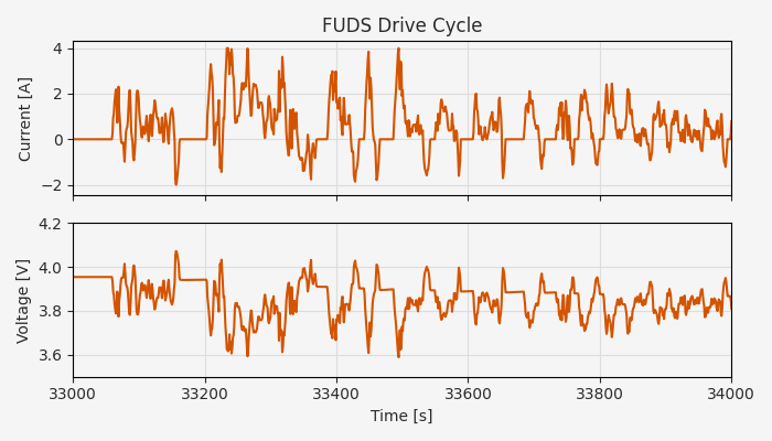
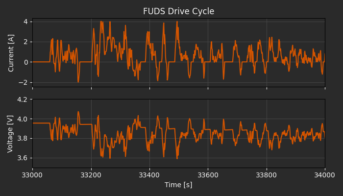
Besides the incremental discharge test, the CALCE dataset has a few different “driving schedule” datasets. These are pre-defined current profiles that are designed to be representative of real-world usage, including:
Federal Urban Driving Schedule (FUDS): A 1370-second simulation of power requirements for city driving, originating in the 1970’s from EPA efforts to standardize mileage testing
US06: A more aggressive EPA profile developed in the 1990’s to approximate more realistic highway driving conditions
Dynamic Stress Test: A 360-second test profile designed by DOE labs specifically to evaluate batteries under dynamic conditions
The CALCE dataset has test data for all of these profiles cycling from 80% charge until full discharge, creating a rich dataset of dynamic conditions across charge levels.
This also offers a great opportunity to test the hypothesis that the ECM will generalize well beyond training conditions. For this demo we’ll fit the model using the first of ~10 FUDS cycles (starting at 80% SOC) and then test the estimated parameters using the remaining FUDS data plus US06 and DST. This will test the model on more aggressive current profiles and on deeper discharge levels than the training set.
We’ll use the Timeseries struct as a convenient way to manage these different datasets - this is basically a small container for input/output data that combines timestamps ts with inputs us and observations ys.
The CALCE Excel files all have the same structure, so they can be processed with a common utility.
def process_drive_cycle(df, t0):
    time = df["Test_Time(s)"].to_numpy()
    current = df["Current(A)"].to_numpy()
    voltage = df["Voltage(V)"].to_numpy()

    dt = np.median(np.diff(time))

    # Invert SOC-OCV curve to estimate initial SOC
    ocv_init = np.interp(t0, time, voltage)
    def ocv_residual(soc):
        return ocv_init - np.polyval(ocv_coeffs, soc)

    # Root-finding with autodiff using initial SOC estimate of 80%
    soc_init = arc.root(ocv_residual, 0.8)
    x0 = np.array([soc_init, 0.0, 0.0])

    # Uniform time grid
    ts = np.arange(t0, time[-1], dt)
    us = np.atleast_2d(np.interp(ts, time, -current))
    ys = np.atleast_2d(np.interp(ts, time, voltage))

    data = arc.sysid.Timeseries(ts=ts, us=us, ys=ys)

    return data, x0


df_fuds = pd.read_excel("calce/SP2_25C_FUDS/11_06_2015_SP20-2_FUDS_80SOC.xls", sheet_name="Channel_1-008", usecols="B,G:J")
fuds_data, x0_fuds = process_drive_cycle(df_fuds, t0=33000)

df_us06 = pd.read_excel("calce/SP2_25C_US06/11_11_2015_SP20-2_US06_80SOC.xls", sheet_name="Channel_1-008", usecols="B,G:J")
us06_data, x0_us06 = process_drive_cycle(df_us06, t0=10500)

df_dst = pd.read_excel("calce/SP2_25C_DST/11_05_2015_SP20-2_DST_80SOC.xls", sheet_name="Channel_1-008", usecols="B,G:J")
dst_data, x0_dst = process_drive_cycle(df_dst, t0=19000)
fig, ax = plt.subplots(2, 1, sharex=True, figsize=(7, 4))

ax[0].plot(fuds_data.ts, fuds_data.us[0, :])
ax[0].set_ylabel("Current [A]")
ax[0].grid()

ax[1].plot(fuds_data.ts, fuds_data.ys[0, :])
ax[1].set_ylabel("Voltage [V]")
ax[1].grid()
ax[1].set_ylim([3.5, 4.2])

ax[0].set_title("FUDS Drive Cycle")
ax[-1].set_xlabel("Time [s]")
ax[-1].set_xlim([33000, 34000])
plt.tight_layout()
plt.show()
Next, split out the training data from the full dataset. Properly, we should not use the training data in evaluation at all, but to keep things simple here (basically, to avoid re-estimating the initial SOC), we’ll use the full FUDS data as the test set.
tf_train = 34500  # 1500 seconds after t0 - approximately one full FUDS cycle
train_data = fuds_data[fuds_data.ts <= tf_train]
dt = train_data.ts[1] - train_data.ts[0]

forward_train = make_forward(train_data.ts, train_data.us)
forward_test = make_forward(fuds_data.ts, fuds_data.us)
Now we are finally ready for the optimization. Beyond reasonable ballpark values for an initial guess, we can also define some plausible parameter ranges to help the optimizer find valid solutions.
model_init = BatteryECM(ocv_coeffs=ocv_coeffs, R0=0.1, R1=0.1, C1=1e5, R2=1e-3, C2=1e3)
lower_bounds = model_init.replace(R0=1e-6, R1=1e-6, C1=1e-6, R2=1e-6, C2=1e-6)
upper_bounds = model_init.replace(R0=1.0, R1=100.0, C1=np.inf, R2=100.0, C2=np.inf)
The optimization itself is a straightforward nonlinear least-squares problem. We’ll use SciPy’s “trust region reflective” algorithm, wrapped in arc.optimize.least_squares to take advantage of autodiff and use struct compatibility. This takes around 30 seconds on a MacBook Pro laptop.
def residuals(model):
    xs_pred, ys_pred = forward_train(model, x0_fuds)
    return ys_pred[0, :] - train_data.ys[0, :]

# Estimate parameters
result = arc.optimize.least_squares(
    residuals,
    model_init,
    bounds=(lower_bounds, upper_bounds),
    options={
        "ftol": 1e-8,
        "xtol": 1e-8,
        "max_nfev": 300,
        "verbose": 2,
    },
    method="trf",
)

model_opt = result.x
Iteration     Total nfev        Cost      Cost reduction    Step norm     Optimality
       0              1         4.3606e-01                                    3.02e+00
       1              2         2.3894e-01      1.97e-01       8.27e+04       1.28e+00
       2              3         1.1838e-01      1.21e-01       1.05e+03       4.83e+02
       3              4         4.3766e-02      7.46e-02       2.10e+03       1.94e+02
       4              5         5.1211e-03      3.86e-02       4.27e+03       2.75e+01
       5              6         2.1276e-03      2.99e-03       5.68e+02       9.06e+00
       6              7         1.9345e-03      1.93e-04       4.42e+03       7.17e-01
       7              8         1.8935e-03      4.11e-05       1.99e+03       1.02e-03
       8              9         1.8868e-03      6.71e-06       6.22e+02       1.56e-04
       9             10         1.8857e-03      1.06e-06       2.51e+02       5.14e-05
      10             11         1.8855e-03      1.81e-07       1.06e+02       1.91e-05
      11             12         1.8855e-03      3.14e-08       4.51e+01       7.50e-06
      12             13         1.8855e-03      5.52e-09       1.90e+01       3.05e-06
      13             14         1.8855e-03      9.55e-10       8.00e+00       1.26e-06
      14             15         1.8855e-03      3.07e-10       3.36e+00       5.27e-07
      15             22         1.8855e-03      0.00e+00       0.00e+00       5.27e-07
`xtol` termination condition is satisfied.
Function evaluations 22, initial cost 4.3606e-01, final cost 1.8855e-03, first-order optimality 5.27e-07.
print("Optimized parameters:")
print(f"\tR0: {model_opt.R0:.3f} Ω")
print(f"\tR1: {model_opt.R1:.3f} Ω")
print(f"\tC1: {model_opt.C1:.3f} F")
print(f"\tR2: {model_opt.R2:.3f} Ω")
print(f"\tC2: {model_opt.C2:.3f} F")
print("\nTime constants:")
print(f"\tτ1: {model_opt.R1 * model_opt.C1:.3f} s")
print(f"\tτ2: {model_opt.R2 * model_opt.C2:.3f} s")
Optimized parameters:
	R0: 0.072 Ω
	R1: 0.022 Ω
	C1: 17069.877 F
	R2: 0.021 Ω
	C2: 873.450 F

Time constants:
	τ1: 373.501 s
	τ2: 18.595 s
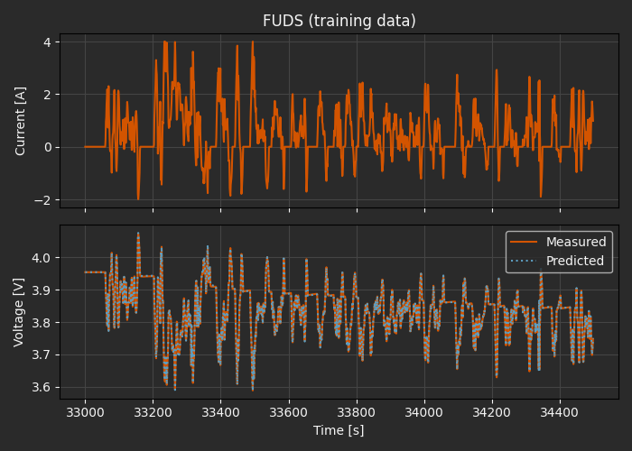
xs_pred, ys_pred = forward_train(model_opt, x0_fuds)
xs_test, ys_test = forward_test(model_opt, x0_fuds)
fig, ax = plt.subplots(2, 1, sharex=True, figsize=(7, 4))
ax[0].plot(train_data.ts, train_data.us[0, :])
ax[0].set_ylabel("Current [A]")
ax[0].grid()
ax[1].plot(train_data.ts, train_data.ys[0, :], label="Measured")
ax[1].plot(train_data.ts, ys_pred[0, :], ':', label="Predicted")
ax[1].set_ylabel("Voltage [V]")
ax[1].grid()
ax[1].legend()
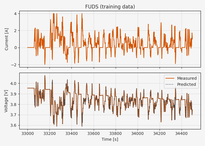
ax[0].set_title("FUDS (training data)")
ax[-1].set_xlabel("Time [s]")
plt.tight_layout()
plt.show()
fig, ax = plt.subplots(2, 1, sharex=True, figsize=(7, 4))

ax[0].plot(fuds_data.ts, fuds_data.us[0, :])
ax[0].set_ylabel("Current [A]")
ax[0].grid()

ax[1].plot(fuds_data.ts, fuds_data.ys[0, :], label="Measured")
ax[1].plot(fuds_data.ts, ys_test[0, :], ':', label="Predicted")
ax[1].set_ylabel("Voltage [V]")
ax[1].grid()
ax[1].legend()

ax[0].set_title("FUDS (full data)")
ax[-1].set_xlabel("Time [s]")
plt.tight_layout()
plt.show()
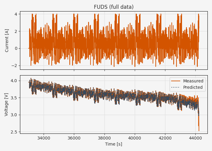
Visually, the fit is overall quite good, but clearly starts to diverge around 10% SOC.
rmse_train = np.sqrt(np.mean((train_data.ys[0, :] - ys_pred[0, :])**2))
print(f"RMSE (train data): {rmse_train*1000:.2f} mV")

def rmse(ys_true, ys_pred, xs_pred):
    rmse = np.sqrt(np.mean((ys_true - ys_pred)**2))

    # Error above 10% SOC
    mask = xs_pred[0, :] > 0.1
    rmse_masked = np.sqrt(np.mean((ys_true[0, mask] - ys_pred[0, mask])**2))

    print(f"RMSE (full data):  {rmse*1000:.2f} mV")
    print(f"RMSE (SOC > 10%):  {rmse_masked*1000:.2f} mV")

rmse(fuds_data.ys, ys_test, xs_test)
RMSE (train data): 1.65 mV
RMSE (full data):  22.49 mV
RMSE (SOC > 10%):  5.44 mV
20-30 mV error levels to full discharge are still quite good, and <10 mV errors are probably suitable for a variety of applications like Kalman filter-based online SOC estimation.
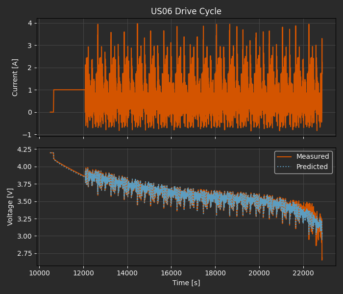
We’ve already loaded the US06 and DST data sets, so extending this validation is straightforward:
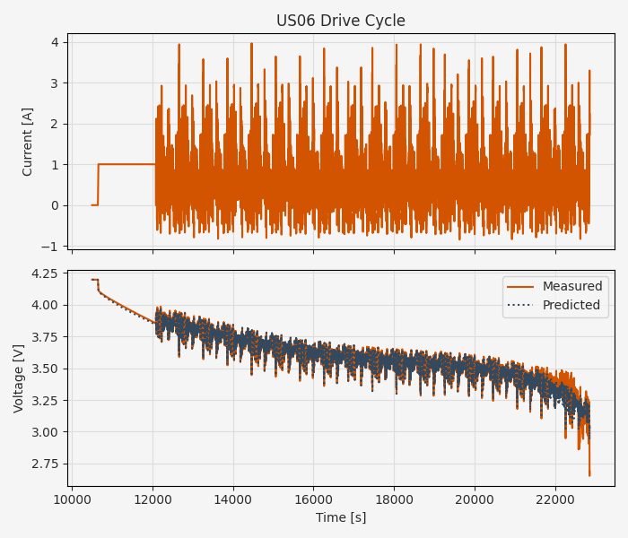
forward_us06 = make_forward(us06_data.ts, us06_data.us)
xs_pred, ys_pred = forward_us06(model_opt, x0_us06)
rmse(us06_data.ys, ys_pred, xs_pred)

fig, ax = plt.subplots(2, 1, sharex=True, figsize=(7, 4))

ax[0].plot(us06_data.ts, us06_data.us[0, :])
ax[0].set_ylabel("Current [A]")
ax[0].grid()

ax[1].plot(us06_data.ts, us06_data.ys[0, :], label="Measured")
ax[1].plot(us06_data.ts, ys_pred[0, :], ':', label="Predicted")
ax[1].set_ylabel("Voltage [V]")
ax[1].grid()
ax[1].legend()

ax[0].set_title("US06 Drive Cycle")
ax[-1].set_xlabel("Time [s]")
plt.tight_layout()
plt.show()
RMSE (full data):  21.45 mV
RMSE (SOC > 10%):  6.15 mV
forward_dst = make_forward(dst_data.ts, dst_data.us)
xs_pred, ys_pred = forward_dst(model_opt, x0_dst)
rmse(dst_data.ys, ys_pred, xs_pred)

fig, ax = plt.subplots(2, 1, sharex=True, figsize=(7, 4))

ax[0].plot(dst_data.ts, dst_data.us[0, :])
ax[0].set_ylabel("Current [A]")
ax[0].grid()

ax[1].plot(dst_data.ts, dst_data.ys[0, :], label="Measured")
ax[1].plot(dst_data.ts, ys_pred[0, :], ':', label="Predicted")
ax[1].set_ylabel("Voltage [V]")
ax[1].grid()
ax[1].legend()

ax[0].set_title("DST Drive Cycle")
ax[-1].set_xlabel("Time [s]")
plt.tight_layout()
plt.show()
RMSE (full data):  25.48 mV
RMSE (SOC > 10%):  6.14 mV
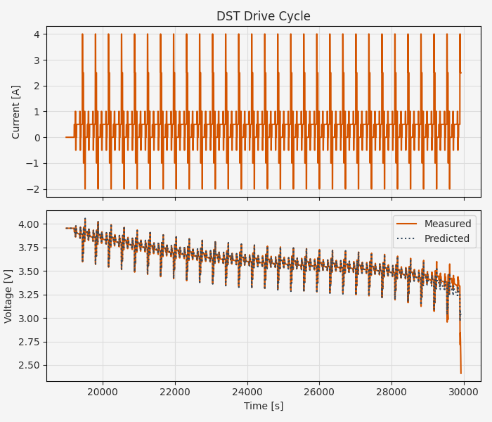
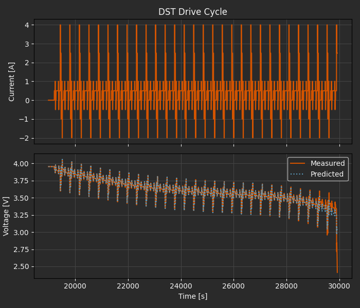
In all cases we have consistent error levels of roughly 5-6 mV down to 10% charge, and 20-25 mV throughout the full operating range, based on fitting to a single incremental pulse test and one cycle of FUDS data.
What we haven’t done here is fully parameterize the model; the equivalent circuit component parameters fluctuate with SOC (especially in the <10% range, as we’ve seen), with temperature, and with battery health. While a simple constant-component model like might be useful for applications like SOC estimation, robust “digital twin”-style monitoring applications likely require broader parameterization.
Beyond Batteries
The point of this tutorial is not only that you can use Archimedes for developing equivalent circuit models of Li-ion batteries (but you can!). More broadely, this is also an example of a full parameter estimation workflow applied to real experimental data.
The key takeaways are:
The choice of model parameterization has a huge impact on how tractable the parameter estimation problem is, and on how well the model generalizes to unseen conditions.
Not all parameters need to be estimated in a single optimization problem. By splitting out the steady-state polynomial estimation from the dynamic system identification, we were able to reduce the more expensive and less convex system ID phase to five parameters while remaining confident in the quality of our steady-state model.
Splitting the data into training and test sets is critical, but must be done with care in order to properly test generalization. We did a little of that here, but we still didn’t test how well our ECM would perform at different ambient temperatures or over the full battery lifespan.
The specific strategies for the Li-ion ECM probably won’t map perfectly to your parameter estimation problem, but these core principle might. There’s often not a one-size-fits-all solution, but domain knowledge, modeling intuition, and as much data as you can get your hands on is the best recipe for success.